Plotting the Wilson distribution

Introduction Full Paper (PDF)

We have discussed the Wilson score interval at length elsewhere (Wallis 2013a, b). Given an observed Binomial proportion p = f / n observations, and confidence level 1-α, the interval represents the two-tailed range of values where P, the true proportion in the population, is likely to be found. Note that f and n are integers, so whereas P is a probability, p is a proper fraction (a rational number).

The interval provides a robust method (Newcombe 1998, Wallis 2013a) for directly estimating confidence intervals on these simple observations. It can take a correction for continuity in circumstances where it is desired to perform a more conservative test and err on the side of caution. We have also shown how it can be employed in logistic regression (Wallis 2015).

The point of this paper is to explore methods for computing Wilson distributions, i.e. the analogue of the Normal distribution for this interval. There are at least two good reasons why we might wish to do this.

The first is to shed insight onto the performance of the generating function (formula), interval and distribution itself. Plotting an interval means selecting a single error level α, whereas visualising the distribution allows us to see how the function performs over the range of possible values for α, for different values of p and n.

A second good reason is to counteract the tendency, common in too many presentations of statistics, to present the Gaussian (‘Normal’) distribution as if it were some kind of ‘universal law of data’, a mistaken corollary of the Central Limit Theorem. This is particularly unwise in the case of observations of Binomial proportions, which are strictly bounded at 0 and 1.

As we shall see, the Wilson distribution diverges from the Gaussian most dramatically as it tends towards the boundaries of the probabilistic range, i.e. where the interval approaches 0 or 1. By contrast, the Normal distribution is unbounded, and continues to plus or minus infinity.

The Wilson score interval (Wilson 1927) may be computed with the following formula.

Wilson score interval (w^–, w⁺) ≡ p + z²/2n ± z√p(1 – p)/n + z²/4n²
1 + z²/n.
(1)

Let us first consider cases where P is less than p. At the lower bound of this interval (P = w^–) the upper bound for the Gaussian interval for P, E⁺, must be equal to p (Wallis 2013a).

We can carry out a test for significant difference between p and P by either

1. calculating a Gaussian interval at P and testing if p is greater than the upper bound, or
2. calculating a Wilson interval at p and testing if P is less than the lower bound.

To consider cases where P is greater than p, we simply reverse this logic. We test if p is smaller than the lower bound of a Gaussian interval for P, or P is greater than the upper bound of the Wilson interval for p. The Gaussian version of the test is called the single proportion z test. It can also be calculated as a goodness of fit χ² test (Wallis 2013a, b).

Excerpt

3.3 Varying p

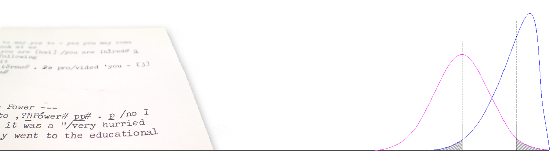
As p tends to 0, we obtain increasingly skewed distributions (Figure 3). The interval cannot be easily approximated by a Normal interval, and the sum of the two distributions is decidedly not Gaussian (‘Normal’).

In Figure 3, note how the mean p is no longer the most likely value (mode).

Figure 3. Plots of Wilson distributions for p = 0.3, 0.1 and 0.0.

In plotting this distribution pair, the area on either side of p is projected to be of equal size, i.e. it treats as a given that the true value P is equally likely to be above and below p. This is not necessarily true! Indeed we might multiply both distributions by the probability of the prior. But this fact should not cause us to change the plot.

Note how, thanks to the proximity to the boundary at zero, the interval for w^– becomes increasingly compressed between 0 and p, reflected by the increased height of the curve.

The tendency to express the distribution like an exponential decline on the least bounded side reaches its limit when p = 0 or 1. The ‘squeezed interval’ is uncomputable and simply disappears.

Contents

1. Introduction
2. Plotting the distribution
   2.1 Obtaining values of w^–
   2.2 Employing a delta approximation
3. Example plots
   3.1 An initial example
   3.2 Properties of the Wilson distributions
   3.3 Varying p
   3.4 Small n
4. Further perspectives on the distribution
   4.1 Percentiles of the Wilson distributions
   4.2 The logit Wilson distribution
   4.3 Continuity-corrected Wilson distributions
5. Conclusions
6. References

Citation (published version)

Wallis, S.A. 2021. Plotting the Wilson Distribution. Chapter 18 in Wallis, S.A. Statistics in Corpus Linguistics Research. New York: Routledge. 297-313.

References

Newcombe, R.G. 1998. Two-sided confidence intervals for the single proportion: comparison of seven methods. Statistics in Medicine 17: 857-872.

Wallis, S.A. 2013a. Binomial confidence intervals and contingency tests: mathematical fundamentals and the evaluation of alternative methods. Journal of Quantitative Linguistics 20:3, 178-208 » Post

Wallis, S.A. 2013b. z-squared: the origin and application of χ². Journal of Quantitative Linguistics 20:4, 350-378. » Post

Wilson, E.B. 1927. Probable inference, the law of succession, and statistical inference. Journal of the American Statistical Association 22: 209-212.

See also

• Full paper (PDF)
• Spreadsheet (Excel)
• Plotting the Clopper-Pearson distribution
• Plotting the Wilson replication distribution
• Plotting the Newcombe-Wilson distribution
• Plotting the distributions of confidence intervals on algebraic operators on proportions
• Plotting confidence intervals on graphs
• Binomial → Normal → Wilson
• Logistic regression with Wilson intervals