Confidence intervals

In this blog we identify efficient methods for computing confidence intervals for many properties.

When we observe any measure from sampled data, we do so in order to estimate the most likely value in the population of data – ‘the real world’, as it were – from which our data was sampled. This is subject to a small number of assumptions (the sample is randomly drawn without bias, for example). But this observed value is merely the best estimate we have, on the information available. Were we to repeat our experiment, sample new data and remeasure the property, we would probably obtain a different result.

A confidence interval is the range of values in which we predict that the true value in the population will likely be, based on our observed best estimate and other properties of the sample, subject to a certain acceptable level of error, say, 5% or 1%.

A confidence interval is like a blur in a photograph. We know where a feature of an object is, but it may be blurry. With more data, better lenses, a greater focus and longer exposure times, the blur reduces.

In order to make the reader’s task a little easier, I have summarised the main methods for calculating confidence intervals here. If the property you are interested in is not explicitly listed here, it may be found in other linked posts.

1. Binomial proportion p

The following methods for obtaining the confidence interval for a Binomial proportion have high performance.

• The Clopper-Pearson interval
• The Wilson score interval
• The Wilson score interval with continuity correction

A Binomial proportion, p ∈ [0, 1], and represents the proportion of instances of a particular type of linguistic event, which we might call A, in a random sample of interchangeable events of either A or B. In corpus linguistics this means we need to be confident (as far as it is possible) that all instances of an event in our sample can genuinely alternate (all cases of A may be B and vice-versa).

These confidence intervals express the range of values where a possible population value, P, is not significantly different from the observed value p at a given error level α. This means that they are a visual manifestation of a simple significance test, where all points beyond the interval are considered significantly different from the observed value p. The difference between the intervals is due to the significance test they are derived from (respectively: Binomial test, Normal z test, z test with continuity correction).

As well as my book, Wallis (2021), a good place to start reading is Wallis (2013), Binomial confidence intervals and contingency tests.

The ‘exact’ Clopper-Pearson interval is obtained by a search procedure from the Binomial distribution. As a result, it is not easily generalised to larger sample sizes. Usually a better option is to employ the Wilson score interval (Wilson 1927), which inverts the Normal approximation to the Binomial and can be calculated by a formula. This interval may also accept a continuity correction and other adjustments for properties of the sample.

Figure 1: Wilson score interval about p = 0.3, with n = 10, obtained by inverting the Normal approximation to the Binomial about P, at 95% interval bounds (w^–, w⁺).

2. Functions of p

Let us consider next a measure that can be expressed as a function of a Binomial proportion.

To compute an interval for a function of p, our first step is to analyse the behaviour of the function over the probabilistic range p ∈ [0, 1]. The simplest way to do this is to plot the function and identify (i) whether it is monotonic over the range, and if it is not, (ii) identify turning points (local maxima or minima).

2.1 Monotonic functions

A monotonic function is one that is either guaranteed to increase or decrease over the range of its parameter (its possible values). See Reciprocating the Wilson interval.

For example:

• fn(p) = p² is monotonic and increasing over the probabilistic range p ∈ [0, 1].
• fn(p) = (p – 0.5)² is non-monotonic over the same range.

A confidence interval for a monotonic function of p can be obtained by simply applying the same function, fn, to its lower and upper bounds. If the function is increasing the transformed bounds will be in the same sequence, but if it is decreasing, the transformed lower bound will be at the upper end:

• increasing: fn(p) ∈ (fn(w^–), fn(w⁺))
• decreasing: fn(p) ∈ (fn(w⁺), fn(w^–))

Monotonic functions have a 1:1 mapping and are invertible, so confidence intervals on these functions inherit these properties. Importantly, if p is significantly different from P it follows that their transformed values are also significantly different:

p ≠ P ↔ fn(p) ≠ fn(P).

If the interval for fn(p) excludes the transformed expected value, fn(P), then the interval for p must exclude P (i.e. p is significantly different from P). A significance test between values of p and P should obtain the same result as a test between fn(p) and fn(P).

Figure 2: Some non-monotonic functions. The lower function has two solutions p for one value of f(p). The stepped function has a plateau where there are many values of p for one value of f(p).

By contrast, a non-monotonic function is inevitably ‘lossy’, that is, if more than one value of p can obtain the score fn(p), it follows that an interval for fn(p) may include scores fn(p′), where p′ is significantly different from p. We must bear this in mind when considering how we test for significant difference and what results may mean.

Some example increasing monotonic functions:

• odds p / (1 – p)
• logit log(p) – (1 – log(p))
• weighting, e.g., frequency f = np (sample size n is ‘given’, and thus a constant)
• addition, e.g., an intercept as in kp + c
• logarithm log_k(p)
• logistic (inverse logit)
• power p^k where k > 0

Some example decreasing monotonic functions:

• reciprocal 1/p, e.g. clause length l = 1/p
• power p^k where k < 0

2.2 Non-monotonic functions

This is all very well, but what if we need to compute a confidence interval for a non-monotonic function?

For example, Binomial entropy can be expressed as the negated sum of a function of a proportion p and its alternate q = 1 – p:

η(p) = –(p.log₂(p) + (1 – p).log₂(1 – p)).

This function is not monotonic, but rises and falls over p ∈ [0, 1]. It has a single turning point, a maximum at p = 0.5, where η(p) = 1.

• If the confidence interval for p excludes this turning point (p = 0.5), then the function can be said to be monotonic within the interval. A conservative interval for η(p) is obtained from these bounds.
• Alternatively, if the interval includes the turning point, the upper bound of the new interval is simply the maximum value for η(p) = mˆ = 1, and the lower bound is the smaller of the two transformed bounds, min(η(w^–), η(w⁺)).

Where a transformed interval contains a turning point we include it, either as a maximum or minimum value.

• maximum: fn(p) ∈ (min(fn(w^–), fn(w⁺)), mˆ)
• minimum: fn(p) ∈ (m̌, max(fn(w^–), fn(w⁺))

Another common example is found in squared error terms of the form (p_i – P_i)², where p_i and P_i are observed and expected proportions respectively. We have a Binomial confidence interval for p_i, but P_i is treated as ‘given’ or constant, so it has no interval. The term has a minimum turning point, m̌ = 0, where p_i = P_i.

3. Functions of multiple proportions

So far we have simply transformed the confidence interval for a single observed Binomial proportion. But many formulae contain more than one independent observed proportion or property, each of which has their own confidence interval. We may wish to obtain intervals on the following:

• difference p₂ – p₁
• sum p₁ + p₂
• ratio p₁ / p₂
• product p₁ × p₂
• power p₁^p₂
• logarithm log_p2(p₁)

3.1 Differences

Newcombe (1998) offers an efficient confidence interval for the difference between two observed proportions, d = p₂ – p₁. Since the intervals for each proportion are independent, he employs a Pythagorean reasoning analogous to the Bienaymé sum of variances rule. The interval widths of the new combined interval are obtained from the hypotenuse of a triangle whose other two sides are the relevant interval widths of each term.

Figure 3: Calculating the lower bound of the Newcombe-Wilson interval, using the Pythagorean Bienaymé formula.

For the difference formula d = p₂ – p₁, we may write:

(w_d^–, w_d⁺) = (–√(u₁^–)² + (u₂⁺)², √(u₁⁺)² + (u₂^–)²),

where u_i^– = p_i – w_i^– and u_i⁺ = w_i⁺ – p_i, and (w_i^–, w_i⁺) are the Wilson score interval bounds for p_i, i ∈ {0, 1}.

This is a zero-based interval, and in this form can be used to simply test whether a difference is significantly different from zero (because d falls outside it).

We may reposition the interval about the difference by subtracting it from d. Now it is an interval on our property, d.

d ∈ (d^–, d⁺) = d – (w_d^–, w_d⁺) = (d – w_d⁺, d – w_d^–).

Note that the resulting upper bound of d, d⁺ = d – w_d^–, is based on the lower bound of p₁ (u₁^–), because p₁ is subtracted in the expression p₂ – p₁, and the upper bound of p₂ (which is positive).

If the resulting interval excludes zero, p₁ and p₂ are significantly different.

3.2 Other mathematical operators

Zou and Donner (2008) generalises this principle to any sound confidence interval of any property on the same scale. Substituting –p₁ for p₁ gives us a sum (see also section 3.4 below), and substituting log(p_i) for p_i gives us a ratio interval. Indeed, armed with the ability to compute confidence intervals on logarithmic functions of p, plus this generalised formula, we can create intervals for all of the above. See An algebra of intervals and Confidence intervals on powers and logs.

Once we can obtain an interval for an effect size, we can compare effect sizes by simply constructing a difference interval and checking if it includes zero.

3.3 Analytical reduction

Before we create a confidence interval for a formula, we need to rewrite the formula in as simple a form as possible.

The key principle is each variable citation = one degree of freedom:

Every independent observed proportion, which would attract an independent confidence interval, has a single degree of freedom, and should be cited once only in the formula.

For example, consider percentage difference, which is typically written

d^% = (p₂ – p₁) / p₁ = d / p₁.

On the basis of this formula we might cite the Newcombe-Wilson difference interval for d (see section 3.1 above) and then use this interval to calculate the ratio formula for d / p₁.

Unfortunately the result is a narrow and excessively conservative interval, because we assumed that d and p₁ were independent, and they are not.

However, we can simplify it even more so that p₁ appears only once:

d^% = p₂/p₁ – 1.

Now we can compute the confidence interval for the ratio of two independent proportions, p₂/p₁, and subtract 1.

This process of simplification is a necessary first step. The best advice is simply to think about the number of different ways the same formula can be expressed, and whether any terms can be ‘cancelled out’. Remember that authors may cite a version of a formula that is easy to explain to the reader: that version may not be optimum for deriving a confidence interval.

3.4 k-constrained summation p₁ + p₂ + … + p_k

If we apply Zou and Donner’s (2008) theorem to the unconstrained sum of independent proportions, we obtain the following interval:

independent sum s ∈ (s^–, s⁺) = (∑p_i – √∑(u_i^–)², ∑p_i + √∑(u_i⁺)²).

In other words, the lower bound is the Pythagorean diagonal of tangential lower bounds; the upper bound is calculated from the upper bounds. We can also substitute any function, fn(p_i), for p_i, provided that we can compute sound confidence intervals on it.

A number of effect size measures, including entropy and goodness of fit ϕ, are computed across discrete Multinomial variables with a closed set of k types or outcomes. In this case, it is necessary to sum a series of error terms, fn(p_i), in the knowledge that the sum of the proportions, ∑p_i, is actually 1. There are k – 1 degrees of freedom. We let κ = k/(k – 1), and scale the sum of variances accordingly.

k-constrained sum s ∈ (s^–, s⁺) = (∑fn(p_i) – √κ∑(u_i^–)², ∑fn(p_i) + √κ∑(u_i⁺)²),

where u_i^– = fn(p_i) – fn(w_i^–) and u_i⁺ = fn(w_i⁺) – fn(p_i).

Tip: When developing an interval, compare its performance for k = 2 with a Binomial derivation for p and q = (1 – p). Although the k-constrained interval will tend to be conservative, it should perform comparably.

4. Performance

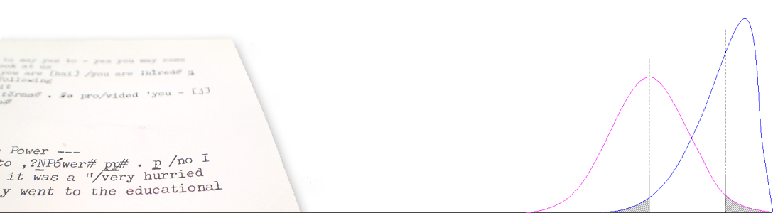
Intervals calculated by these methods are far superior to conventional methods that erroneously assume that the probability density function of an interval is Normal (and symmetric) on some scale. With the exception of the logit (log odds) function, intervals about p (Figure 1) or functions of p are not Normal; when two intervals are combined, a derived interval is also unlikely to be Normal. We need not perform a complex evaluation to reveal this: all we need to do is plot the performance of the interval over the range of p, or permutations of p₁, p₂, etc.

However, Zou and Donner’s theorem does introduce a performance cost in the form of increased Type I errors. This is the error of assuming a difference to be significant when it is not. If we aim for an error level of 0.05 (say), even if we employ the continuity-corrected Wilson score interval for p, a small additional error appears. The performance of proportions in combination may deteriorate, allowing more errors to creep in, especially for small n.

Fortunately, we have found that multiplying the continuity correction term by 1.5 vastly reduces these errors, to a level comparable with Yates’ famous test.

5. Conclusions

This brief post is not intended as a complete account of all possible derivations of confidence intervals. I have not addressed the derivation of intervals on Cramér’s ϕ, for example. With the exception of an initial mention of Clopper-Pearson, I have avoided mention of computational search-based methods. Similarly, there are other adaptations apart from continuity correction that may be applicable for small populations or where instances are not properly random by drawn from contiguous text (random text samples). You will find a discussion of these elsewhere on this blog.

Rather, my intention in writing this post was to give the reader a route in to a set of methods which offer the promise of efficient calculation, good accuracy and a high level of generalisation.

A reader new to the world of confidence intervals will note how these algebraic methods allow us to create a large number of new intervals and thus new tests. A property with an associated confidence interval may be appreciated as observable subject to a predictable level of uncertainty, this uncertainty being expressed by the interval. In contrast, traditional null hypothesis significance testing (NHST) tends to separate descriptive measures and testing procedures, and this kind of evaluation is generally obscured from the research user. This makes interpreting results and carrying out further tests (such as meta-tests comparing repeat runs of the same experiment) much more difficult.

Our methods are also generalisable to confidence intervals on measures other than the Binomial proportion, such as the ratio of two t-distributed natural numbers or positive Reals.

This blog also contains a number of posts exploring the probability density distribution (pdf) ‘shape’ of these confidence intervals. These plots show that for small sample sizes at least, these methods often create distributions that are only occasionally approximately Normal.

References

Newcombe, R.G. (1998). Interval estimation for the difference between independent proportions: comparison of eleven methods. Statistics in Medicine, 17, 873-890.

Wallis, S.A. (2013). Binomial confidence intervals and contingency tests. Journal of Quantitative Linguistics, 20:3, 178-208. » Post

Wallis, S.A. (2021). Statistics in Corpus Linguistics Research. New York: Routledge.

Wilson, E.B. (1927). Probable inference, the law of succession, and statistical inference. Journal of the American Statistical Association 22: 209-212.

Wallis, S.A. (forthcoming). Accurate confidence intervals on Binomial proportions, functions of proportions and other related scores. » Post

Zou, G.Y. & A. Donner (2008). Construction of confidence limits about effect measures: A general approach. Statistics in Medicine, 27:10, 1693-1702.

See also

• Binomial confidence intervals and contingency tests
• Reciprocating the Wilson interval
• An algebra of intervals
• The confidence of entropy – and information
• Confidence intervals on pairwise ϕ statistics
• Confidence intervals on powers and logs
• Confidence intervals on goodness of fit ϕ scores
• Confidence intervals for Cohen’s h
• Continuity correction for risk ratio and other intervals