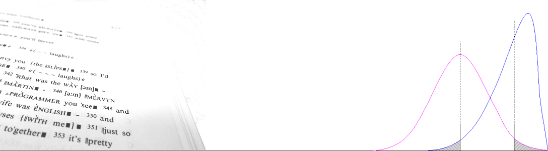
So: you’ve got some data, you’ve read up on confidence intervals and you’re convinced. Your data is a small sample from a large/infinite population (all of contemporary US English, say), and therefore you need to estimate the error in every observation. You’d like to plot a pretty graph like the one below, but you don’t know where to start.

Of course this graph is not just pretty.
It depicts a pattern whereby two synchronically distinct uses become four over time. Note that for any pair of points across a diachronic contrast we can immediately identify the following:
- non-overlapping intervals must be statistically distinct (a significant difference);
- if any point falls within the interval of another, it cannot be significantly distinct (a non-significant difference);
- in all other cases we need to carry out a 2 × 2 test (either Yates’s χ² test or the Newcombe-Wilson continuity-corrected test) to check.
Probabilities drawn from the same sample sum to 1. To compare points in competition synchronically you should use a single sample z test instead of a 2 × 2 test.
In this case, the 1960s data does not significantly distinguish the rates for quotative and interpretive uses of think because the p value for the quotative use is within the interval for the interpretive. A quick check with the 2 × 2 spreadsheet finds that
- the initial fall (from 1920s to 1960s) for ‘cogitate’ uses is significant but
- intention does not change significantly over time (note how the curved line can be misleading), and
- quotative uses significantly increase their share from the 1960s to 2000s.
Other changes can be easily identified in the graph. Note that this graph expresses semasiological (meaning distribution) change, not onomasiological (choice of alternates) change, and results are therefore indicative. We can’t conclude that speakers in later texts increasingly preferred to employ think in a quotative way, without considering this question relative to the opportunity to employ quotative constructions. See Choice vs. use.
Let us discuss how we arrived at this graph.
Step by step
We want to plot the observed probability p with Wilson score interval error bars. We can’t use the Gaussian interval (some values are zero) and anyway, as other posts clarify, it is wrong to do so!
- First we gather the raw data. We need to identify the raw frequencies, f, and the relationship between the different data series. Does it make sense to take proportions out of the total frequency, n? What should the baseline be for any change?
- If we use the total number of cases of think, n, as a meaningful baseline, we can obtain a set of semasiological probabilities for each frequency, p = f / n.
- Next we calculate basic Wilson score interval terms. This is the most complicated step and can be broken down into two components for simple calculation.
- Wilson adjusted centre p′ = p + z²/2n
1 + z²/n, and - Wilson standard deviation s′ = √p(1 – p)/n + z²/4n²
1 + z²/n,
where z = zα/2, the critical two-tailed value of the standard Normal distribution for error level α. We could simplify each expression further and pre-calculate the Wilson denominator [1 + z²/n] for every cell.
- Wilson adjusted centre p′ = p + z²/2n
- We can now calculate the upper and lower bound of the interval in absolute terms:
- Wilson score interval (w–, w+) = (p′ – z.s′, p′ + z.s′).
- Finally we can work out the upper and lower bounds relative to the probability p. Excel likes these both to be positive, so we have the following:
- Wilson relative error bars (u–, u+) = (p – w–, w+ – p).
We can also create Wilson functions, WilsonLower and WilsonUpper, for w– and w+. So for the two-tailed interval we might write
w– = WilsonLower(p, n, α/2), and w+ = WilsonUpper(p, n, α/2).
You can also use the continuity-corrected formula for the Wilson score interval. The conventionally-stated formula is equation (7) in (Wallis 2013) and is implemented in the 2 × 2 spreadsheet. (It is also implemented in the spreadsheet for this example.)
However, more recently I realised it can be calculated with Wilson functions, which is the most intuitive (and least error-prone) method. In simple terms, all we do is move the observed p out by ± 12n.
w–cc = WilsonLower(p – 12n, n, α/2), and w+cc = WilsonUpper(p + 12n, n, α/2).
Note: Since p – 12n may be less than zero, we also need to set WilsonLower to return 0 if the proportion parameter < 0, so we may write w–cc = WilsonLower(max(p – 12n, 0), n, α/2). We perform the equivalent correction for WilsonUpper.
The continuity-corrected interval is slightly more conservative, and corresponds to Yates’s 2 × 1 χ² test. For most plotting purposes, however, the standard Wilson interval is usually perfectly adequate. For more discussion on this point, see Correcting for continuity.
References
Levin, M. 2013. The progressive in modern American English. In Aarts, B., J. Close, G. Leech and S.A. Wallis (eds). The Verb Phrase in English: Investigating recent language change with corpora. Cambridge: CUP. » Table of contents and ordering info
Wallis, S.A. 2013. Binomial confidence intervals and contingency tests: mathematical fundamentals and the evaluation of alternative methods. Journal of Quantitative Linguistics 20:3, 178-208 » Post
See also
- Excel spreadsheet
- Change and certainty: plotting confidence intervals (2)
- Reciprocating the Wilson interval
- Binomial confidence intervals and contingency tests
- Binomial → Normal → Wilson
- Correcting for continuity
