Binomial confidence intervals and contingency tests

Abstract Paper (PDF)

Many statistical methods rely on an underlying mathematical model of probability which is based on a simple approximation, one that is simultaneously well-known and yet frequently poorly understood.

This approximation is the Normal approximation to the Binomial distribution, and it underpins a range of statistical tests and methods, including the calculation of accurate confidence intervals, performing goodness of fit and contingency tests, line-and model-fitting, and computational methods based upon these. What these methods have in common is the assumption that the likely distribution of error about an observation is Normally distributed.

The assumption allows us to construct simpler methods than would otherwise be possible. However this assumption is fundamentally flawed.

This paper is divided into two parts: fundamentals and evaluation. First, we examine the estimation of error using three approaches: the ‘Wald’ (Normal) interval, the Wilson score interval and the ‘exact’ Clopper-Pearson Binomial interval. Whereas the first two can be calculated directly from formulae, the Binomial interval must be approximated towards by computational search, and is computationally expensive. However this interval provides the most precise significance test, and therefore will form the baseline for our later evaluations.

We consider two further refinements: employing log-likelihood in computing intervals (also requiring search) and the effect of adding a correction for the transformation from a discrete distribution to a continuous one.

In the second part of the paper we consider a thorough evaluation of this range of approaches to three distinct test paradigms. These paradigms are the single interval or 2 × 1 goodness of fit test, and two variations on the common 2 × 2 contingency test. We evaluate the performance of each approach by a ‘practitioner strategy’. Since standard advice is to fall back to ‘exact’ Binomial tests in conditions when approximations are expected to fail, we simply count the number of instances where one test obtains a significant result when the equivalent exact test does not, across an exhaustive set of possible values.

We demonstrate that optimal methods are based on continuity-corrected versions of the Wilson interval or Yates’ test, and that commonly-held assumptions about weaknesses of χ² tests are misleading.

Log-likelihood, often proposed as an improvement on χ², performs disappointingly. At this level of precision we note that we may distinguish the two types of 2 × 2 test according to whether the independent variable partitions the data into independent populations, and we make practical recommendations for their use.

Introduction

Estimating the error in an observation is the first, crucial step in inferential statistics. It allows us to make predictions about what would happen were we to repeat our experiment multiple times, and, because each observation represents a sample of the population, predict the true value in the population (Wallis 2013).

Consider an observation that a proportion p of a sample of size n is of a particular type.

For example

• the proportion p of coin tosses in a set of n throws that are heads,
• the proportion of light bulbs p in a production run of n bulbs that fail within a year,
• the proportion of patients p who have a second heart attack within six months after a drug trial has started (n being the number of patients in the trial),
• the proportion p of interrogative clauses n in a spoken corpus that are finite.

We have one observation of p, as the result of carrying out a single experiment. We now wish to infer about the future. We would like to know how reliable our observation of p is without further sampling. Obviously, we don’t want to repeat a drug trial on cardiac patients if the drug may be adversely affecting their survival.

Excerpt

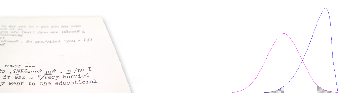
The correct characterisation [of the interval about p] is a little counter-intuitive, but it can be summarised as follows. Imagine a true population probability, which we will call P. This is the actual value in the population. Observations about P will be distributed according to the Binomial. We don’t know precisely what P is, but we can try to observe it indirectly, by sampling the population.

The interval equality principle with Normal and Wilson intervals: the lower bound for p is P. [The upper and lower bounds of the Normal interval about P are E⁺ and E^–, the bounds of the Wilson interval about p are w⁺ and w^–.]

Given an observation p, there are, potentially, two values of P which would place p at the outermost limits of a Gaussian interval about P [i.e. around 0 and 6]. See above. What we can do, therefore, is search for values of P which satisfy the formula used to characterise the Normal approximation to the Binomial about P.

Now we have the following definitions:

pop. mean μ ≡ P,
pop. standard deviation σ ≡ √P(1 – P) / n,
pop. confidence interval (E^–, E⁺) ≡ (P – z.σ, P + z.σ).

The formulae are the same but the symbols have changed. The symbols μ and σ, referring to the population mean and standard deviation respectively, are commonly used. This population interval identifies two limit cases where p = P ± z.σ.

Consider now the confidence interval around the sample observation p. We don’t know P in the above, so we can’t calculate this imagined population confidence interval. It is a theoretical concept! However the following interval equality principle must hold, where e^– and e⁺ are the lower and upper bounds of a sample interval for any error level α:

e^– = P₁ ↔ E₁⁺ = p where P₁ < p, and
e⁺ = P₂ ↔ E₂^– = p where P₂ > p.

If the lower bound for p (labelled e^–) is a possible population mean P₁, then the upper bound of P₁ would be p, and vice-versa. Since we have formulae for the upper and lower intervals of a population confidence interval, we can attempt to find values for P₁ and P₂ which satisfy p = E₁⁺ = P₁ + z.σ₁ and p = E₂^– = P₂ – z.σ₂.

With a computer we can perform a search process to converge on the correct values. The formula for the population confidence interval above is a Normal z interval about the population probability P. This interval can be used to carry out the z test for the population probability. This test is equivalent to the 2 × 1 goodness of fit χ² test, which is a test where the population probability is simply the expected probability P = E/n.

Fortunately, rather than performing a computational search process, it turns out that there is a simpler method for directly calculating the sample interval about p. This interval is called the Wilson score interval (Wilson, 1927).

Contents

1. Introduction
2. Computing confidence intervals
   2.1 The ‘Wald’ interval
   2.2 Wilson’s score interval
   2.3 The ‘exact’ Binomial interval
   2.4 Continuity correction and log-likelihood
3. Evaluating confidence intervals
   3.1 Measuring error
   3.2 Evaluating 2 × 1 tests and simple confidence intervals
4. Evaluating 2 × 2 tests
   4.1 Evaluating 2 × 2 tests against Fisher’s exact test
   4.2 Evaluating 2 × 2 tests against paired exact Binomial test
5. Conclusions

• Preprint (PDF)

Citation

Wallis, S.A. 2013. Binomial confidence intervals and contingency tests: mathematical fundamentals and the evaluation of alternative methods. Journal of Quantitative Linguistics 20:3, 178-208. DOI:10.1080/09296174.2013.799918

• ePublication (Taylor & Francis online)

References

Sheskin, D.J. 1997. Handbook of Parametric and Nonparametric Statistical Procedures. Boca Raton, Fl: CRC Press.

Wallis, S.A. 2013. z-squared: the origin and application of χ². Journal of Quantitative Linguistics 20:4, 350-378. » Post

Wilson, E.B. 1927. Probable inference, the law of succession, and statistical inference. Journal of the American Statistical Association 22: 209-212.

See also

• Testing tests
• Binomial algorithm snippets
• z-squared: the origin and application of χ²
• 2 × 1 and 2 × 2 χ² tests (Excel spreadsheet)
• Plotting the Wilson distribution
• Further evaluation of Binomial confidence intervals