Introduction
Back in 2010 I wrote a short article on the logistic (‘S’) curve in which I described its theoretical justification, mathematical properties and relationship to the Wilson score interval. This observed two key points.
- We can map any set of independent probabilities p ∈ [0, 1] to a flat Cartesian space using the inverse logistic (‘logit’) function, defined as
- logit(p) ≡ log(p / 1 – p) = log(p) – log(1 – p),
- where ‘log’ is the natural logarithm and logit(p) ∈ [-∞, ∞].
- By performing this transformation
- the logistic curve in probability space becomes a straight line in logit space, and
- Wilson score intervals for p ∈ (0, 1) are symmetrical in logit space, i.e. logit(p) – logit(w–) = logit(w+) – logit(p).


The logit function is entirely reversible, so we can translate any linear function, y = mx + c, on the logit scale back to the probability scale using the logistic function:
- logistic(x) = 1 / (1 + e–(mx + c)).
Since m is the gradient of the line in logit space, and c is a fitting constant, it is possible to conceive of m as equivalent to a size of effect measure: the steeper the gradient, the more dramatic the effect. The coefficient of fit, r², is the inverse of a significance test for the fit, so a high r² means a close fit.
This is the rationale used by the method most conventionally referred to as ‘logistic regression’, more accurately logistic linear regression for multiple independent variables. This is the conventional ‘black box’ approach to logistic regression. This relies on a number of mathematical assumptions, including:
- IVs are on a Real or Integer scale, like time (or can be meaningfully approximated by an Integer, such as ‘word length’ or ‘complexity’); and
- logit relationships are linear, i.e. the dependent variable can be fit to a model, or function, consisting of a series of weighted factors and exponents of some or all of the supplied independent variables (a straight line in n-dimensional logit space). Consider extending the second graph above in a third dimension so the line declines into the page to see what I mean.
However, properly conceived, logistic regression can do more than that. As we shall see, there are good reasons for believing that relationships may not be linear on a logit scale.
Performing regression
One of the ideas I had at that time is that it would be possible to perform regression in logit space by minimising least square errors over variance, where ‘variance’ is approximated by the square of the Wilson interval width. Any function in logit space can then be converted back to a function in p space by the logistic function.
- As anyone who paid attention in maths class knows, linear regression is a method for finding the best line through a set of data points and operates by minimising the total error e between each point and the proposed line. So if all your data neatly lines up, then a line might pass through them all and we have a regression score, r², of 1. Usually, however, we have a bit of a scatter. A cloud, in which any line would be as good as any other, will score 0.
- The error is computed by the square of the difference between each point and the line, and then totalled up, so, for a series of probabilities, px, and a function, P(x), representing the ideal population value:
- error e = ∑(P(x) – px)².
- A variation of this method takes account of a situation where different data points are considered to be of greater certainty than others. In this case we divide the squared errors by the square of the standard deviation for each point, Sx² (also called the variance):
- standard deviation Sx ≡ √P(x)(1 – P(x))/N(x).
- error e = ∑(P(x) – px)² / Sx².
My proposal was to swap the standard deviation on P(x) for the Wilson width on px (in logit space). The Wilson interval width is an adjusted error for sample probability values. It contains a constant factor, zα/2, but this cancels out. This method is both efficient and highly generalisable.
- The method is very efficient.
- The Wilson width only needs to be calculated once for all px values, whereas the standard deviation must be calculated on P(x), which changes all the time during fitting. (Computing standard deviations using the Gaussian approximation to the Binomial on observations px obtains the mathematically incorrect ‘Wald’ interval.)
- Regression is guaranteed to converge, as we don’t have a moving target.
- It maximises the fit for the estimate of the crossing point (c, where p = 0.5) and gradient m in that region.
- It is also generalisable to other functions. Here we fit a straight line, P(x) = m(x – k), but a polynomial or other function could readily be employed.
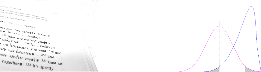
- This estimate of variance is not merely symmetric. It turns out that the distribution of the logit Wilson function is approximately Normal, see Plotting the Wilson distribution.
An example
The following examples draw on data from Bowie and Wallis (2016), in which we used this approach to regress time series data.
Here is some test data from that paper which illustrates the method. (If you are interested, it is the probability of selecting OUGHT to-infinitive perfect, ‘to HAVE Ved’, out of the ‘modality’ verbs OUGHT, HAVE and BE over 20 decades from COHA — not exactly an alternation pattern!)
The dashed straight line represents the line selected by the algorithm. Upper and lower lines track the upper and lower bounds of the 95% Wilson interval.

One problem is that if p = 0 or 1, logit(p) is infinite. However, if you think about it, the interval width is also infinite, so the point may safely be ignored. This is the data for ‘BE to HAVE Ved’.

Finally, here is the same data and regression lines plotted on a probability scale and presented with Wilson score intervals.

Footnote
This example bears out the earlier observation that we could conceivably apply functions other than straight lines to this data. The second logit graph (lower line in the graph above) may better approximate to a non-linear function.
From my perspective, I prefer not to over-fit data to regression lines. I tend to think that it is better that researchers visualise their data appropriately.
Data may converge to a non-linear function on a logit scale (i.e. not be logistic on a probability scale) for at least two reasons.
- There are multiple ecological pressures on the linguistic item (in this case, proportions of lemmas out of a set of to-infinitive perfects in COHA) or it may be because the item is not free to vary from 0 to 1, which is sometimes the case. We have already noted that these forms are not true alternates.
- The forms may be subject to multinomial competition. In this case, we have three competing forms, a 3-body situation which would not be expected to obtain a logit-linear (logistic) outcome. For simplicity, I plotted two curves, but it is wise to bear in mind that the logistic is a model of a simple change along one degree of freedom, and a three-way variable has two degrees.
It is sometimes worth comparing regression scores, r², numerically (all fitting algorithms try to maximise r²). If we simply wish to establish a direction of change, the threshold for a fit can be low, with scores above 0.75 being citable. On the other hand if we have an r² of 0.95 or higher we can meaningfully cite the gradient m.
Generally, however, conventional thresholds for fitting tend to be more relaxed than those applied to confidence intervals and significance tests because the underlying logic of the task is quite distinct. Several functions may have a close fit to the given data, and we cannot say that one is significantly more likely than another merely by comparing r² scores.
Citation (extended version)
Wallis, S.A. 2021. Competition Between Choices Over Time. Chapter 11 in Wallis, S.A. Statistics in Corpus Linguistics Research. New York: Routledge. 178-194.
References
Bowie, J. and Wallis, S.A. (2016). The to-infinitival perfect: a study of decline. In Werner, V., Seoane, E., and Suárez-Gómez, C. (eds.) Re-assessing the Present Perfect, Topics in English Linguistics (TiEL) 91. Berlin: De Gruyter, 43-94.
