Introduction
Statistical tests based on the Binomial distribution (z, χ², log-likelihood and Newcombe-Wilson tests) assume that the item in question is free to vary at each point. This simply means that
- If we find f items under investigation (what we elsewhere refer to as ‘Type A’ cases) out of n potential instances of the item, the statistical model of inference assumes that it must be possible for f to be any number from 0 to n, which we can write as f ∈ [0, n].
- Both observed proportion p = f / n and population proportion P are therefore expected to fall in the probabilistic range, P = [0, 1].
Note that this constraint is a mathematical one. All we are asserting is that the true proportion in the population P (and thus the probability of randomly selecting the item) could conceivably range from 0 to 1.
This property is not limited to onomasiological studies which require strict alternation of types with constant meaning. In semasiological studies, where we evaluate alternative meanings of the same word, these tests may also be used. This is because it is conceivable that the proportion of a meaning in a sample can be any value from 0 to 1.
However, it is also common in corpus linguistics to see evaluations carried out against a baseline that contains terms that simply cannot plausibly be exchanged with the item under investigation. The most obvious example is statements of the following type: “linguistic item x increases per million words between category 1 and 2”, with reference to a log-likelihood or χ² significance test to justify this claim. Rarely is this appropriate.
Some terminology: We will use Types A and B to represent validly alternative items. So if Type A is the use of modal shall, most words will not alternate with shall. Type B cases would be those that can alternate with shall (e.g. modal will in certain contexts).
The remainder of cases (other words) are, for the purposes of our study, not evaluated. We will term these invariant cases Type C, because they cannot replace Type A or Type B.
In That vexed problem of choice we explained that introducing such ‘Type C’ cases into an experimental design conflates opportunity and choice, causing the potential range of proportions to be less than 1, and worse still, often to vary between subsamples.
In this post we make a further observation. This methodological error also makes the statistical evaluation of variation more conservative. Not only may we mistake a change in opportunity as a change in the preference for the item, but we also weaken the power of statistical tests and tend to reject significant changes (in statistics jargon, “Type II errors”).
This problem of experimental design far outweighs differences between methods for computing statistical tests. In brief, an increase in non-alternating ‘Type C’ cases makes a test more conservative, so significant variation which would be identified with a more theoretically-relevant baseline, will tend to be missed with a more general one. This is despite the fact that eliminating Type C cases yields a smaller sample. This conservatism arises from the fact that by introducing invariant terms we are gradually undermining the mathematical assumptions of the Binomial model and its approximations (Gaussian, log-likelihood, etc.).
A mathematical demonstration
We can demonstrate the problem of conservatism with rising n using the ‘Wald’ Gaussian approximation to the Binomial interval. As we have noted elsewhere, the Wald formula is not a good approximation to the ‘exact’ Clopper-Pearson interval. As we shall see in the next section, a similar result is obtained with the Wilson score interval, which is a better approximation. But it has one advantage for our initial explanatory purposes. It is symmetric (p – e, p + e), and therefore we only need concern ourselves with one variable: the error interval width e = zα/2.√p(1 – p)/n.
The question we are concerned with is simply this. What happens to e as n increases by gaining Type C cases, but the number of cases where alternation is actually possible (Types A vs. B) stays the same?
Let us observe a fixed number of both types, f Type A cases and f′ Type B cases. We now increase n by adding a further number of Type C cases which could not alternate with A or B. As we know, significance testing involves comparing observed and expected frequencies (f and F respectively) or probabilities (p, P). Whether we employ a Wilson interval, χ² or a single-sample z test, at the heart of the test we compare p = f / n with P = F / n. (We have seen how other tests are built on these foundations.)
Consider what happens to the width of the error interval e if n increases but everything else stays the same. The following table shows what happens to e with f = 60. As the sample size n increases, the chance of randomly selecting a Type A case, p = f / n, falls. The interval width e on the same scale also shrinks, so at first glance, the test becomes less conservative.
| n | 100 | 316.23 | 1,000 | 3,162.28 | 10,000 |
| f | 60 | 60 | 60 | 60 | 60 |
| p | 0.6 | 0.189737 | 0.06 | 0.018974 | 0.006 |
| e | 0.096018 | 0.043215 | 0.014719 | 0.004755 | 0.001514 |
| e / pmax | 0.096018 | 0.136658 | 0.147193 | 0.150371 | 0.151362 |
Table. Scaled Gaussian interval widths, e / pmax, for f = 60 genuine Type A, f′ = 40 Type B cases and increasing numbers of non-alternating Type C cases making up the difference.
But this observation is misleading. This estimate assumes that in fact these additional members of the sample can be replaced with Type A. The Binomial model of variation assumes that at its maximum, p = 1 and f = n.
But this cannot happen if some instances in our data set are Type C. These new cases do not alternate with either A or B. The maximum value for f is still f + f′ = 100. Therefore p can only reach a maximum of pmax, defined simply as
pmax = p({A, B} | {A, B, C}) = (f + f′) / n.
We could call pmax the prior probability of opportunity, i.e. the chance that the choice A vs. B is available. It defines the possible range of variation at any given time.
To compare interval widths across sample sizes, therefore we must first divide the width e by pmax. The idea is illustrated by the following figure.

This method allows us to plot the following figures. The figure below plots the Gaussian scaled interval width e / pmax over exponentially increasing n for different values of f. For n = 100, there are no Type C cases in the data, pmax = 1 and the error interval is not distorted.

As the baseline size n increases, the interval expands, and corresponding statistical tests become more conservative.
- The impact of rising n differs with initial frequency f. Consider the line for f = 5, i.e. where the true rate is 5%, or five items out of a baseline of n cases. The line is almost flat, indicating that rising n barely changes the likelihood of obtaining a significant result. However as f increases to occupy a greater share of the original n = 100 cases (20, 40, 60, 80, 95), the error interval increases by a greater fraction. This means that the ‘freedom to vary’ assumption matters more for observed proportions closer to 50% (f = 50) than 0%.
- Note that this problem affects majority types (types whose proportion exceeds 50%) to a greater extent than minority types. With a simple binary choice, the probability of Type B cases is 1 – p. If Type A is in a minority out of A and B, then B is a majority type, and likely to be subject to a conservative assessment of significance. As you can see from the figure, the interval for f = 95 increases more than four-fold with rising n.
For transparency, the calculations for the Gaussian and Wilson intervals are presented in this spreadsheet.
An example
There are 885,436 words in the Diachronic Corpus of Present-Day Spoken English (DCPSE), of which 150 are first person declarative shall, and 136 are will. The overall percentage of shall f = 150×100/286 = 52%. However, were we to employ a word baseline, there would be 885,150 Type C cases (words that are neither shall nor will). There are approximately 3,095 Type C cases for every single alternating case (A or B).
On the same scale, the 95% Gaussian error for f (we have employed a ‘Wald’ approximation for simplicity here: error intervals for observations should always use a Wilson-based interval, see below) rises from 0.0578 calculated against the alternating cases, to approximately 0.0839 calculated against the number of words, an increase of 45%.
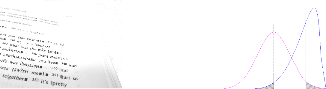
However, “an increase of 45%” underestimates the scale of the problem. This increase is a change in the interval width, not the tail area under the curve. The test is actually now ten times more conservative than it should be. Recall that the error level is the proportion of the area under the Normal curve in the tail area, and it turns out that this area α = 0.0044 rather than the figure we wanted, 0.05!

We can compute the tail area using the cumulative Normal distribution function. The standardised version of this function has a mean of 0 and a standard deviation of 1. This statement deserves a little explaining.
The standard Normal distribution function is the probability density function of the Normal distribution. That means it returns the theoretical probability of observing a particular Real number x, assuming a mean of 0 and a standard deviation of 1. It may be used to plot the Normal distribution and it generates the famous ‘bell curve’ (below).

In other words, it returns the height of any given horizontal point x along this curve.
Standard Normal ϕ(x) = 1
√2π e–x²/2,
for any value of x from –∞ to +∞.
The cumulative version of this function calculates the area under the curve from –∞ to x. Since it is continuous, to add up the area we employ an integral (the flattened ‘S’ symbol below). If you did calculus at school you might recognise what is happening here. If you did not, do not worry — just remember that the function adds up the heights in the equation above along the x axis to calculate the area.
Standard cumulative Normal Φ(x) = ∫x
–∞ 1
√2π e–t²/2 dt.
However, a standardised function is not very useful. Its main use is as a comparison for z scores, i.e. to test if the standard cumulative Normal Φ(z) ≤ α/2. What we want is a generalised cumulative Normal function for any given mean and standard deviation. This would allow us to calculate the lower tail area below a point x for any Normal curve.
Fortunately, we can transform this function by the simple arithmetic below. The mean, x¯, is subtracted from x and the standard deviation scales the difference.
Cumulative Normal Φ(x, x¯, s) = Φ((x – x¯) / s).
All we need do now is substitute the lower bound for x = p – e/pmax and the mean x¯ = p. We calculated the standard deviation s when we calculated e. The area from –∞ to x is the lower tail area, so we multiply this by 2 to obtain the error level α.
Recalibrated error level α = 2 × Φ(p – e/pmax, p, s).
In this case, α turns out to be 0.0044, rather than the figure the model was intended to have, 0.05. As a result of using a per-million-word baseline for investigating shall / will variation in DCPSE, significance tests are of the order of ten times more conservative than they should be. Widening the error interval width causes the remaining tail area to shrink.
An increase in interval width is worrying enough. But such a statement understates the loss of sensitivity of tests. The tail area should be 2.5%, but as a result of the Type C cases being admitted into the sample, the actual area is less than a tenth of this, at around 0.22%.
The last figure plots what happens to the error level α in our model for different values of f as n increases. This indicates that the greater the true proportion p, the more rapidly α will decline.

Other interval calculations
These results are not an artefact of the Gaussian formula for an expected probability P. They are fundamental to the statistical inference model of contingent variation (i.e. the Binomial model). Methods for calculating the interval range for observations p obtain essentially the same pattern. The figure below plots Wilson and log-likelihood intervals alongside the ‘Wald’ Gaussian, for f = 95. Again, the correct value is at the far left hand side (where n = N = 100). These intervals are asymmetric and have a different upper and lower bound (Wallis 2013). Lower and upper bounds swap over when p = 0.5 (here, at n = f × 2 = 190).

Conclusions
The statistical model underpinning Binomial-type tests and intervals assumes that observed frequencies f can take any value from 0 to n. However, many corpus linguistics researchers use a baseline for n that includes many cases that do not alternate, a common example being found in the use of ‘per million word’ baselines. Most phenomena in linguistic data are not as frequent as words, and cannot plausibly be so!
In this post, we considered what happens to the statistical model if a baseline includes non-alternating terms. In our model, the baseline includes n – (f + f′) invariant Type C terms, but the true freedom to vary is limited to a ceiling of N = f + f′ = 100.
The outcome is inevitable: if frequency counts include large numbers of invariant terms and yet we employ statistical models that assume that the item in question is free to vary, then not only are these tests used inappropriately, we can predict that they will tend to be conservative. A corollary is that if we have a small number of invariant terms then these tests should generally be fine. This mathematical observation outweighs differences between interval computations.
In brief:
The selection of a particular statistical computation (Gaussian, Wilson, log-likelihood etc.) is less important than the question of correctly specifying the experimental design, i.e. in using this type of test, restricting data to a set of types that could plausibly range from 0 to 100%.
Appropriate data could include strict choice-alternates expressing the same meaning (onomasiological change), but might also include different meanings for the same word, string or structure (semasiological change). See Choice vs. use. The item must be free to vary, i.e. that it is conceivable that a sample could have 100% of any single given type.
This analysis is in addition to the “envelope of variation” problem, i.e. that invariant Type C cases may also vary in number over the contrast, such as time, under study. See That vexed problem of choice.
Type C cases should ideally be eliminated, but if this is not possible they should be minimised (another way of looking at the graphs above is that the problem is reduced as n approaches 100).
The presence of large numbers of invariant Type C terms would impact on many other statistical models that assume that the item being evaluated is free to vary. For example, this problem also undermines the use of logistic models (S-curves), effectively turning logistic regression into a type of linear principal component analysis.
References
Wallis, S.A. 2013. Binomial confidence intervals and contingency tests: mathematical fundamentals and the evaluation of alternative methods. Journal of Quantitative Linguistics 20:3, 178-208. » Post
