Coping with imperfect data

Introduction

One of the challenges for corpus linguists is that many of the distinctions that we wish to make are either not annotated in a corpus at all or, if they are represented in the annotation, unreliably annotated. This issue frequently arises in corpora to which an algorithm has been applied, but where the results have not been checked by linguists, a situation which is unavoidable with mega-corpora. However, this is a general problem. We would always recommend that cases be reviewed for accuracy of annotation.

A version of this issue also arises when checking for the possibility of alternation, that is, to ensure that items of Type A can be replaced by Type B items, and vice-versa. An example might be epistemic modal shall vs. will. Most corpora, including richly-annotated corpora such as ICE-GB and DCPSE, do not include modal semantics in their annotation scheme. In such cases the issue is not that the annotation is “imperfect”, rather that our experiment relies on a presumption that the speaker has the choice of either type at any observed point (see Aarts et al. 2013), but that choice is conditioned by the semantic content of the utterance.

Suppose you have preliminary results, obtained with a rough-and-ready search, and these obtain a statistically significant result. However you suspect that there are some errors in the annotation, or that some cases that have been included in your search (or excluded from your search) should not be counted. What do you do?

1. Is it worth manually checking every example, of which there may be hundreds, if not thousands?
2. Do you do nothing, i.e. rely on the results you have so far?
3. Or is there a third option?

One of the advantages of obtaining a mathematical understanding of significance tests and confidence intervals, which this blog attempts to convey, is that it offers us a mathematical answer to this problem. Without this type of reasoning, the only truly reliable solution would be to choose the first option above. First, you would broaden the search sufficiently to include false negatives (i.e. cases that perhaps should be included but were missed). Second, you then manually check every example found to get an accurate count.

In practice, the majority of papers I see (and this sin is common in automatic “statistical” analyses of data, because it is extremely difficult to “drill down” to the source examples) is just to rely on results obtained from (often crude) searches, i.e. the second option. But if you have no idea as to how large the misclassification risk is, you cannot be sure of your results.

Fortunately, there are some simple solutions to this problem.

Estimating the effect of misclassification

In some situations, for example where the number of cases overall are small, I have to recommend that researchers use Option 1. But if your dataset is large, checking every example is likely to be very costly in terms of time. There are two different versions of Option 3, and they are suitable for slightly different situations.

1. Test the worst-case scenario. Check every example. This is quick and easy to explain (bear in mind you need to explain to your readers what you have done).
2. Factor in estimates of error, with confidence intervals. You only need review a random subsample of your data.

In this blog post I discuss adapting tests with a single degree of freedom. With some care, the methods discussed may be extended to more complex r × c tests, but this is rarely necessary in practice.

An example

Wallis (2012) compares the distribution of sequential decisions of the same type, a form of complexity. In one experiment we compare two types of operations on postmodifying clauses (clauses that modify a noun phrase head such as the ship [by the jetty]):

1. embedded clauses the ship [by the jetty [in the harbour]]. The second clause modifies the previous head, the jetty.
2. sequential clauses the ship [by the jetty] [with the green funnels]. The second clause modifies the original head the ship.

Employing the parse annotation in the corpus, we obtain graphs like this.

Sequential vs. embedded NP postmodifying clauses, from Wallis (2012).

This graph tells us that the probability of embedding a second postmodifying clause, p(2), is significantly lower than the probability of adding a single postmodifying clause, p(1). The same is true for sequential postmodifying clauses. However, if we examine the circled area, what can we say about the two second-stage probabilities? We compare embedding and sequentially modifying the original head. The raw data from corpus queries reveals the following:

	F(1)	F(2)	p(2)
embedded	9,881	227	0.0230
sequential	10,112	166	0.0164

The frequency columns, F(x), refer to the total number of cases that have at least x clauses, so the probability of adding a clause at stage x is simply p(x) = F(x)/F(x-1). For simplicity, we can import this data into the 2 × 2 χ² spreadsheet (hint: F(2) is a row of cells, F(1) is a row of totals) and apply a Newcombe-Wilson test (Wallis 2013) to confirm that these observations are significantly different. (Note: in the paper we employ a separability test to compare the falls in p rather than p itself.) The two columns now look like this.

	IV:	embedded		sequential
add	F(2)	227		166
¬add	F(1)-F(2)	9,654		9,946
Total	F(1)	9,881		10,112

But can we rely on the annotation? Are all cases that are analysed as double sequential clauses correctly analysed? What about ambiguous examples, such as the ship by the jetty next to the lighthouse?

Testing the worst-case scenario

Given that p(embed,2) > p(seq,2), the worst-case scenario is that ambiguous embedded cases should correctly be analysed as sequential. This would reduce the probability p(embed,2), increase the probability p(seq,2), and thereby reduce their difference – making a significant difference harder to obtain.

NB. This example considers the misclassification of examples by the independent variable (IV), but the same logic applies to a dependent variable (DV). See below.

We therefore check the embedded cases for ambiguity. We do not need to check the sequential ones. By examining all 227 cases, 7 out of 227 cases are sufficiently ambiguous to suggest that they could be analysed as sequential. We simply re-apply the significance test by subtracting this number from the embedded column and adding it to the sequential one. Reapply the significance test with these adjusted figures, and it is still significant. For clarity, I have highlighted the changing values in the table.

	IV:	embedded		sequential
add	F(2)	220	→	173
¬add	F(1)-F(2)	9,654		9,946
Total	F(1)	9,874	→	10,119

Note that this method requires no elaborate calculations. All that we need to do is consider the impact of misclassification on the experimental design. Indeed, you can quickly adjust the values in the 2 × 2 χ² spreadsheet.

NB. In this instance, misclassified instances mutually substitute (two postmodifying clauses must be analysed as either embedded or sequential). If cases do not alternate, then misclassified cases are merely eliminated rather than transferred.

The method errs on the side of caution. If a case is ambiguous, we transfer it (or eliminate it if appropriate). It also presumes that it is feasible to check all cases manually, which is possible for 227 cases, but is unlikely to be feasible if cases run into the thousands.

Factoring in estimates of errors

The second method derives from the first, but is used when you have too many cases to check manually.

If you cannot be sure of the exact number of ambiguous or erroneous cases that are included in your data, you can take a random subsample and evaluate those. Suppose we find that in a random subsample of 100 out of our 227 cases, 5 are potentially incorrectly included. This factor, which we will call p(err), is an observed 5% error, or an expected 11.35 out of 227 cases in error. For simplicity, henceforth we will refer to p(embed) and p(seq) when we discuss the second-stage probabilities.

Unfortunately, we cannot easily adapt a contingency table, as above, because we have to factor in the confidence interval associated with our error estimate. Instead we’ll modify the Newcombe-Wilson test. We compute a 95% Wilson interval on p(err), applying Singleton’s adjustment for a finite population. This obtains the interval (0.0240, 0.1011) or an error range of 2.4% to 10.1%. This interval is justified on the basis that a random sample of 100 cases will have an error, but the sample is a true subset of our original observation.

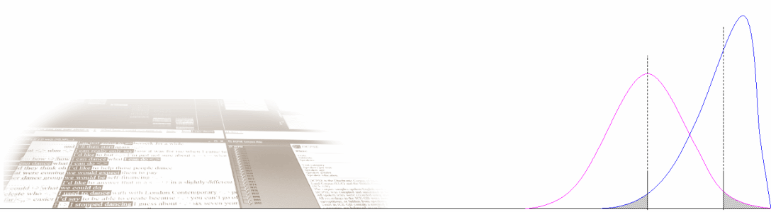
The next figure sketches the basic idea. First, we move p(embed) assuming the worst case scenario (subtracting 11.35 from 227) as above. Second, we estimate a new confidence interval, combining the confidence intervals for p(embed) and p(err), as shown below. We have used colours to distinguish between the two intervals.

The basic idea: combine error estimate (dark red) with observation (blue) to obtain new interval (purple).

Stage 1: recomputation for p(embed)

1. The modified observation is:
   • p(embed) = (227 – 11.35) / (9,881 – 11.35) = 0.0218.
   • 95% Wilson interval = (0.0191, 0.0249).
   • lower interval width: y^–(embed) = p(embed) – w^–(embed) = 0.0218 – 0.0191 = 0.0027. We are interested in the lower interval because we are expecting to remove misclassified cases.
2. The error estimate for the observation p(embed) is:
   • p(err) = 5/100 = 0.05.
   • 95% interval = (0.0240, 0.1011).
   • upper interval width y⁺(err) = 0.1011 – 0.05 = 0.0511.
3. Next we need to scale the error estimate. The error is based on a subsample. The error can only occur in the embedded cases. So this error must be scaled by the first probability: p(embed) × p(err).
   • scaled upper interval width y⁺′(err) = 0.00117.
   • We are interested in the upper interval because this represents the maximum number of misclassified embedded cases we might remove.
4. We incorporate the observed error using the sum of squares (Bienaymé formula):
   • lower interval width for p(embed): y′^–(embed) = √y^– (embed)² + y⁺ ′(err)² = 0.0029.

Note that as a result of this process the lower interval width increases from 0.0027 to 0.0029.

Stage 2: transfer to p(seq)

As, in this instance, misclassified cases transfer to the sequential set, we also apply the error term y⁺′(err) to the upper bound of p(seq, 2).

• modified observation after transfer: p(seq) = (166 + 11.35) / (10,112 + 11.35) = 0.0175.
• modified upper interval width: y⁺(seq) = w⁺(seq) – p(seq) = 0.0027.
• upper interval width for p(seq): y′⁺(seq) = √y⁺ (seq)² + y⁺ ′(err)² = 0.0029.

This stage is omitted if misclassified cases are eliminated rather than transferred.

Stage 3: revised difference test

These new interval widths can be incorporated in a revised Newcombe-Wilson test.

• p(embed) – p(seq) > √y′^– (embed)² +y′⁺ (seq)².
• 0.0043 > 0.0042, i.e. a significant difference.

Note that we have traded the effort in checking 127 cases for a more complex calculation, but a well-constructed spreadsheet can make the entire exercise fairly simple.

NB. To get you started, I have added a page to the Wilson sample-population spreadsheet.

Modifying Wilson intervals as a result of manually evaluating a subsample of the higher observation. In this case data is transferred from p(embed) to p(seq). The Newcombe-Wilson test is performed on the modified intervals.

The result is significant (just), which is fine. But if the result of reviewing a subsample was non-significant, you would still have the option of reviewing more cases.

One of the benefits of a mathematical understanding of inferential statistics is that it allows us to decide whether we have enough data to obtain a significant result. In this case, it allows us to decide whether it is worth reviewing more cases, and obtain a more accurate error estimate with a smaller confidence interval.

This method converges on the worst-case scenario when the subsample becomes the sample (y⁺(err) = 0).

Dependent variable alternation

In the experiment we discussed above, the impact of misclassification applied between two independent observations (embedded vs. sequential), i.e. values of the independent variable (IV). So if a case was misclassified as embedded, it would be correctly analysed as sequential, and vice-versa. Cases are therefore transferred across the values of the IV. Where cases are eliminated but not reclassified they do not transfer, and we do not carry out Stage 2 above.

Sometimes, misclassified cases transfer between values of the dependent variable (DV). Suppose that instead of considering whether embedded postmodification was correctly analysed as two sequential postmodifiers, instead we decided that actually some cases of two-deep embedding might be correctly one level deep after all. This misclassification error would cause transfer within the embedded column, like this:

DV:		embedded		sequential
added:	↓	220		166
not added:		9,661		9,946
Total		9,881		10,112

Note that probabilities sum to 1 across the DV, but are independent across the IV. What happens in one column does not affect the other. The total number of cases does not change.

• If we review all cases, we simply adapt the table and perform the appropriate test.
• If we review a subsample, we perform Stage 1 and Stage 3 above without changing the value of n(embed). Note that if the DV has two values, p and q, then q = 1-p and a significant difference for p is also a significant difference for q. This means we do not have to recalculate the amended confidence interval for q.

In conclusion

When we evaluate linguistic data from a corpus quantitatively, we risk forgetting that our data must be correctly identified qualitatively in the first place. The process of abstracting data from a corpus and presenting it in a regular dataset is prone to a range of errors. The two principal problems that you will need to address in this way are

• Misclassifying cases within the data set (identifying Type A as Type B and vice-versa).
• Including cases in the dataset that should be excluded (false positives), e.g. non-alternating cases. (The problem of false negatives is addressed by drawing the net wider – and then excluding cases.)

The solution is slightly different in either situation. If cases should not be included at all, we simply need to consider the effect of excluding them. On the other hand, if some cases are misclassified, then the loss on one side of the equation must be compensated by a gain in the other. When we attempt to improve on preliminary results, we can take a short-cut by recognising that the most important question is whether there is evidence that undermines our first observation.

So if we see a significant difference, we should focus on evidence that might contradict this observation. If we can eliminate this possibility, the results are safe to report.

NB. Note that the reverse is not true: the methods we discuss in this blog post attempt to make an initial significant observation more robust by increasing the margin of error or reducing the difference observed. The only way to refine an experiment yielding a non-significant result to obtain a significant one would be by identifying cases more precisely.

The approach described above can be used for erroneous cases and ambiguous ones, although we would normally report tables with figures adjusted by correcting erroneous classification.

It is possible to argue that for ambiguous cases one might estimate the likelihood of cases falling in each category (by default: halving the error estimate). However, we have taken a worst-case approach and assumed that all ambiguous cases were in fact errors.

Naturally, these methods do not prevent us going further and making our experiment more accurate, and obtain a more precise true rate for the sample, but the minimum criterion is to ensure that significant results are not a mere artefact of poor annotation and abstraction methods in the first place. Our first obligation is to ensure our results are robust and sound.

There really is no excuse for not checking your data.

Citation (substantially extended)

Wallis, S.A. 2021. Conducting Research with Imperfect Data. Chapter 16 in Wallis, S.A. Statistics in Corpus Linguistics Research. New York: Routledge. 263-276.

References

Aarts, B., Close, J, and Wallis, S.A. 2013. Choices over time: methodological issues in investigating current change. » ePublished. Chapter 2 in Aarts, B., Close, J, Leech, G. and Wallis, S.A. (eds.) The Verb Phrase in English. Cambridge: CUP. » Table of contents and ordering info

Singleton, R. Jr., B.C. Straits, M.M. Straits and R.J.McAllister, 1988. Approaches to social research. New York, Oxford: OUP.

Wallis, S.A. 2012. Capturing patterns of linguistic interaction. London: Survey of English Usage, UCL. » Post

Wallis, S.A. 2013. Binomial confidence intervals and contingency tests: mathematical fundamentals and the evaluation of alternative methods. Journal of Quantitative Linguistics 20:3, 178-208 » Post

See also

• Wilson sample-population spreadsheet
• Robust and sound?
• Inferential statistics and other animals
• Binomial confidence intervals and contingency tests
• z-squared: the origin and application of χ²