Plotting entropy confidence interval distributions

Introduction

In this blog post, I will discuss the distribution of confidence intervals for the information-theoretic measure, entropy.

One of the problems we face when reasoning with statistical uncertainty concerns our ability to mentally picture its shape. As students we were shown the Normal distribution and led to believe that it is reasonable to assume that uncertainty about an observation is Normally distributed.

Even when students are introduced to other distributions, such as the Poisson, the tendency to assume that uncertainty is expressed as a Normal distribution (‘the Normal fallacy’) is extremely common. The assumption is not merely an issue of weak mathematics and poor conceptualisation: since Gauss’s famous method of least squares relies on Normality, this issue affects fitting algorithms and error estimation applied to non Real variables, such as the one discussed here.

As a general rule, whenever I have developed methods for computing confidence intervals I have done my best to plot, not just the interval bounds (the upper or lower critical threshold at a given error level) but the probability density function (pdf) distribution of the interval bounds. The results are often surprising, and gain us fresh insight into the intervals we are using.

Entropy is an interesting case study for two reasons. First, there are two methods for computing the two-valued measure, one more precise but less generalisable than the other. Second, like many effect sizes, the function involves a non-monotonic transformation, which has important implications for how we conceptualise uncertainty and intervals. (Indeed, so far I have not published the equivalent distributions for goodness of fit ϕ or diversity, both of which engage the same type of transformations.)

First we will do some necessary recapitulation, so bear with me.

Preliminaries: entropy, and intervals for the single proportion

In The confidence of entropy – and information we introduced the standardised or ‘normalised’ entropy measure η ∈ [0, 1] obtained from Equation (1).

entropy η ≡ – Σ
i p_i.log_k(p_i) = – 1
ln(k) Σ
i p_i.ln(p_i), (1)

for k values for competing proportions p_i, i ∈ {1, 2,… k}, Σp_i = 1, with k – 1 degrees of freedom. If p_i = 0 or 1, the term p_i.ln(p_i) is zero.

On the face of it, this function seems quite simple. One might imagine that the distribution of uncertainty would be approximately bell-shaped (Normal) about the score. Indeed, for large n, the distribution pair does approach this shape, as we shall see.

To compute confidence intervals for a formula like this, we first compute Binomial confidence intervals for each of the probability terms p_i. Whereas one might employ an ‘exact’ Clopper-Pearson computation, the Wilson score interval p ∈ (w^–, w⁺), which may be computed with and without continuity corrections for each p_i is an excellent alternative that is more efficient to compute.

Wilson interval bounds (Wilson 1927) can be considered as a three-parameter function, with parameters proportion p, sample size n and error level α. We may write

w^– = WilsonLower(p, n, α/2),
w⁺ = WilsonUpper(p, n, α/2), (2)

where

Wilson score interval (w^–, w⁺) ≡ p + z²/2n ± z√p(1 – p)/n + z²/4n²
1 + z²/n,
(3)

and z is the two-tailed critical value of the Normal distribution at error level α (written z_α/2 in full). Continuity-corrected intervals are easily obtained by substituting

w^–_cc = WilsonLower(max(0, p – 12n), n, α/2),
w⁺_cc = WilsonUpper(min(1, p + 12n), n, α/2).(2′)

In the previous blog post, we derived two methods for obtaining confidence intervals for entropy. The first was a special Binomial case for k = 2; the second was a more general Multinomial case for a variable with any number of outcomes k.

Method 1. Binomial entropy interval, k = 2

In the Binomial case, we let p = p₁. Then, since p₂ = 1 – p₁, Equation (1) becomes

η(p) = –(p.log₂(p) + (1 – p).log₂(1 – p)), (4)

and η(p) = 0 if p = 0 or 1.

This is a symmetric non-monotonic function of the single proportion, p, with a maximum at p = 0.5, and two minima at p = 0 and 1.

As the function can be determined by a single parameter, all we need to do is suitably transform the interval bounds. Were η(p) to be monotonic, we could simply transform bounds η(w^–), η(w⁺) and order the two scores appropriately.

However, since the function is not monotonic, we have to detect and manage the maximum. We may define an interval (η_b^–,η_b⁺) where

η_b^– = min(η(w^–), η(w⁺)),

η_b⁺ = (5){ η(w⁺)
η(w^–)
1 if w⁺ < 0.5
if w^– > 0.5
otherwise.

See The confidence of entropy for more information. To compute continuity-corrected intervals we simply substitute w^–_cc and w⁺_cc into the formula.

Note. We will employ the subscript ‘b’ in this blog post (for Binomial method) to distinguish intervals from the Multinomial case (labelled ‘m’).

Figure 1. Plotting the upper and lower confidence interval bounds for binary entropy obtained by Equation (5).

The resulting interval bounds may be plotted alongside entropy η for varying p as in Figure 1. Intervals are read vertically, as illustrated. Note how the two generating functions change places and the maximum does not exceed 1. This type of plot reveals how the interval bounds behave, but it does not tell us about how uncertainty is distributed, or, to put it another way, where the population value is more likely to be. In order to do this we need to plot the interval function for particular values of p and thus η(p).

Method 2. Multinomial entropy interval, k > 2

Method 1 is limited to base 2 entropy scores, so for a more general Multinomial solution we employ Zou and Donner’s (2008) theorem to the sum of k terms with k – 1 degrees of freedom (see Wallis forthcoming). Although we have an accurate deterministic method for k = 2, we can also apply this formula to the Binomial condition, which we do here for the purposes of comparison.

First, we compute intervals for the inner term in Equation (1), which we will call ‘inf(p_i)’.

inf(p_i) = –p_i.log_k(p_i). (6)

Like entropy, the ‘inf’ function is non-monotonic, rising to a maximum of mˆ = 1/e ≈ 0.367879. We can compute intervals for Equation (6), inf(p_i) ∈ (h_i^–, h_i⁺), using a similar approach as before:

h_i^– = min(inf(w_i^–), inf(w_i⁺)),

h_i⁺ = (7){ inf(w_i⁺)
inf(w_i^–)
inf(mˆ)  if w_i⁺ < mˆ
if w_i^– > mˆ
otherwise.

Next, we compute an interval for entropy by computing interval widths for the k-constrained sum by summing the square of interval widths and multiplying by a factor, κ = k/(k – 1):

u^– = √κ Σ(inf(p_i) – h_i^–)², and u⁺ = √κ Σ(inf(p_i) – h_i⁺)², (8)

This results in the following interval (which we will label with the subscript ‘m’ for the Multinomial method):

(η_m^–, η_m⁺) = (max(η – u^–, 0), min(η + u⁺, 1)). (9)

Again, for more discussion of this method and its implications, see The confidence of entropy. Previously, we noted that the Binomial interval was less conservative than the Multinomial, although the intervals tended to have more and more comparable performance as n increased.

We include ‘max’ and ‘min’ functions to avoid the phenomenon of Multinomial overshoot, where the interval becomes wider than is possible. We can see examples of this in Figure 2.

Figure 2. Multinomial intervals (green) and Binomial intervals (blue), for varying p and sample size n. Note the pronounced overshoot above η = 1. There is also a very small lower bound overshoot near η = 0.

Plotting the distribution of entropy intervals

A confidence interval bound for a property such as entropy, η, can be thought of as the point on its scale beyond which the tail area of uncertainty (the area beyond the interval) equals the error level α. Except where η = 0 or 1, the interval will have an upper and lower bound, but these are unlikely to be symmetric. We perform the computation for each interval independently.

To plot the interval distribution we employ the delta approximation method described in Wallis (2021: 297). For more information see Plotting the Wilson distribution.

Suffice it to say, this is a flexible mathematical technique that converts an interval formula, like those above, to a distribution curve, revealing where the majority of expected values of the true value in the population are predicted to be. The proportion p is usually a natural fraction of n, i.e. p = f / n where f ∈ {0, 1, 2,… n}.

We obtain a height h(η′, α) for each interval bound η′ and for a sequence of error levels α. We compute the distributions for each bound separately. The area under each bound should sum to 1.

Note. As we shall see, where a distribution is ‘cropped’ at 1, it will generate a sharp peak at 1, although arguably this is an artifact of the plotting algorithm. We might argue that this peak represented a legitimate overshoot (see Plotting the Wilson replication distribution). Where η⁺ > 1, the cropped interval includes 1, i.e. η ∈ (η^–, 1]. Alternatively we might better conceive of it as representing cases where the uncertainty was folded back.

All computations are performed in Excel. The latest version of the spreadsheet avoids macros, which  would make it less portable than would be ideal.

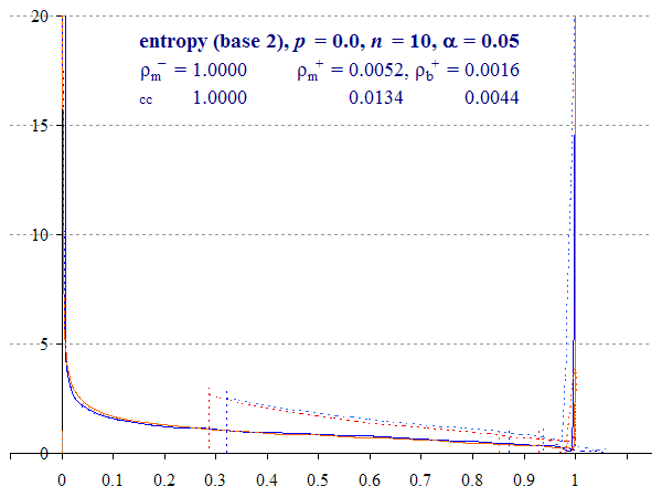
Figure 3 shows interval distributions for the case where p = 0.1 and n = 10. This is a very small sample size to estimate entropy, and so generates a wide interval. If you think about it, the probability range is effectively halved, since η(p) reaches a maximum of 1 at p = 0.5, and then declines as p increases further (hence the graph for p = 0.1 is also the graph for p = 0.9).

We compute normalised entropy η(p) = 0.4690. The two-tailed Binomial interval with α = 0.05 is (η_b^–, η_b⁺) = (0.1293, 0.9733) whereas the Multinomial interval (η_m^–, η_m⁺) is (0.1097, 0.9876). With a continuity correction applied, these intervals become (0.0473, 0.9951) and (0.0168, 1) respectively.

To make the figure a little easier to read, we have highlighted the interval bounds with coloured triangles and labelled them appropriately (e.g. ‘η_b^– _cc(0.05)’ means the Binomial lower bound with continuity correction where α = 0.05 (i.e. for a 95% confidence interval).

Figure 3. Pdf distributions of entropy intervals (η^–, η⁺) by Binomial and Multinomial methods, with and without corrections for continuity. Sample size n = 10, p = 0.1 (or 0.9), η(p) = 0.4690, with two-tailed intervals for α = 0.05 indicated.

A number of features are visible in this graph.

Continuity-corrected intervals begin at η(p ± 12n) for the Binomial (0.2864, 0.6098), whereas uncorrected intervals appear to be a continuous curve. A small rounding error introduced by Equation (9) sees the Multinomial interval begin slightly beyond this point (the point where α = 1, see Plotting the Wilson distribution).

The corrected intervals are ‘squeezed’ into the remaining space, so the curve tends to be higher.

The lower bounds for all four intervals are greater than zero in all cases, unless p = 0.

In this case, the uncorrected Binomial upper bound is just below 1 (0.9936), but all intervals are cropped by the global maximum, causing the method to place the excess at 1, which is visualised as a spike. As we discussed in The confidence of entropy, both methods are conservative. We can plot the distribution of the uncropped interval function in order to witness this overshoot phenomenon.

• Binomial folding. Since it is directly computed, we can plot the distribution of ‘folded’ Binomial scores. In other words, Equation (4) computes both bounds, but does not order the lower or higher, or crop an upper bound at 1, which we do with Equation (5). If we plot these uncropped intervals, the remaining curves turn back on themselves, below 1 (see also Figure 1). But this entire area should be added to the curve at 1.
• Multinomial overshooting. The Multinomial method averages the upper and lower bounds by a sum-of-squares calculation on the interval widths. Part of the curve can exceed, or ‘overshoot’, the range of η ∈ [0, 1]. Now, these are impossible scores, because no true value of entropy in the population, Η, could fall outside this range. Again, this area is added to the excess.

Note: Both methods generate a spike at 1, and Multinomial overshoot also exhibits a second spike beyond 1. What do these represent? They are artifacts of the plotting method. Non-monotonic functions tend to return a large number of cases at the turning point, in this case the maximum, 1. As a result, when we compute an area under the curve, we may generate an infinite column of zero width! In addition, range constraints (‘max’ and ‘min’ functions) substitute limits for the residual overshoot area. The second overshoot spike is in fact due to the turning point of the ‘inf’ function (Equation (7)).

If we permute values of p from 0 to 1, entropy increases to 1 as p reaches 0.5 and then falls back to 0 as a mirror image (see Figure 1). Consequently each distribution for p > 0.5 is the exact same pattern as for the alternate proportion q = 1 – p < 0.5.

Animation 1. Distributions of intervals computed by permuting observed entropy from p = 0.0 to 0.5 and back (noting η(0.4) = η(0.6)), with a small sample size, n = 10. Includes Multinomial overshoot (blue) and folded Binomial (orange).

Calculating residual areas

In Plotting the Wilson replication distribution we discussed the concept of interval residuals, the area under the curve where interval functions generated scores outside the possible range of true values Η ∈ [0, 1]. Whereas some functions might generate overshoot erroneously (the Wald interval being a good example), in other cases this excess may be unavoidable.

We can compute the area of the Binomial fold, ρ_b⁺, by searching for the value of α where the Wilson upper bound is 0.5, i.e. at the turning point of Equation (5). The simplest way to do this is to employ Equation (2). If p < 0.5, we apply Equation (10). If p > 0.5, we solve for q = 1 – p.

Find α where WilsonUpper(p, n, α/2) = 0.5. (10)

We can also find each area of lower and upper Multinomial overshoot by solving for α with a search procedure. We remove ‘min’ and ‘max’ limits from Equation (9) and identify the cross-over point where the bound equals zero or 1. For example, to find the lower bound we search for α where η – u^– = 0.

These methods yield the computed areas in Table 1. Each figure is the proportion of the area of the respective distribution, i.e. the upper interval in the case of ρ⁺, etc.

	ρ–	ρ+	ρ–cc	ρ+cc
Binomial		0.0114		0.0268
Multinomial	0.0000	0.0406	0.0113	0.0841

Table 1. Residual areas ρ (separate tails) for cases of Binomial folding and Multinomial overshoot visible in Figure 1, p = 0.1, n = 10. See also Animation 1.

As we discussed, Binomial folding only occurs at the upper end of the range, when η = 1 is within the distribution. Multinomial overshoot can be found at both upper and lower ends of the range [0, 1], and will be more conservative (and approximate). Multinomial overshoot is invariably treated as simply returning the limit, hence the ‘spike’ at 1 in Figure 1. The overshoot spike is due to the ‘inf’ function (see above).

With the exception of the continuity-corrected Multinomial upper bound, ρ_m⁺ _cc, all are smaller than α = 0.05, and so 95% interval bounds are within the range of Η.

The impact of sample size

The pdf distributions in Figure 3 (and their permutation in Animation 1 above) are spread across most of the entire entropy range, due to the small sample size for estimating entropy.

Indeed, for the same data, interval widths are a factor of between 2 and √2 larger than the equivalent for the single proportion, p. This is equivalent to a sample size for the simple proportion of no larger than n = 10/2 = 5. This seems intuitively plausible: the variable reaches its maximum at p = 0.5 rather than 1, and loses information due to this ‘doubling up’.

So, what happens if we increase n?

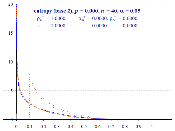
Consider Figure 4, calculated with sample size n = 40. Now, with p = 0.1 (or 0.9) the distribution has no detectable overshoot at either end, and no spike.

We see a close fit between the two methods for the upper interval. For the lower interval, the two methods also converge, but there is a greater discrepancy here, with the Multinomial method being slightly more conservative.

Finally, we can see that the impact of the continuity correction reduces, which we would expect with increasing n.

Figure 4. Distributions of upper and lower bounds of entropy η for n = 40, p = 0.1 or 0.9, η(p) = 0.4690, showing convergence between Binomial and Multinomial methods for larger samples. The upper bound intervals at α = 0.05 are almost identical, whichever method is employed.

This does not mean that the distributions converge equally over the entire range, however. A greater discrepancy between the upper bound distributions can be observed as p tends towards 0.5.

Thus Figure 5, which plots the same graph for p = 0.25, shows that the two methods of calculation of the upper bound differ, with the two-tailed 95% Multinomial interval upper bound reaching 1 with or without a correction for continuity. Being calculated directly, rather than smoothed by Zou and Donner’s theorem, the Binomial method is less conservative, even with the continuity correction.

Figure 5. Distributions for upper and lower entropy bounds, p = 0.25 or 0.75 and n = 40. Note how the lower bounds converge while the upper bounds now differ. Binomial folding is negligible (ρ_b⁺ = 0.0016, ρ_b⁺ _cc = 0.0027), but Multinomial overshoot is in excess of a = 0.05 (ρ_m⁺ = 0.0550, ρ_m⁺ _cc = 0.0787).

Binomial and Multinomial lower intervals appear to converge, although if we increase p towards 0.5 and η = 1, the methods diverge again (see Animation 3 below). The two methods have comparable performance, but the Multinomial method involves a smoothing assumption which errs on the side of caution.

We will end this section with two animations. Animation 2 plots distributions with a constant entropy (η(p) = 0.4690), with increasing sample size n, doubling each time from n = 10. This illustrates ever-more ‘Normal-like’ performance as sample sizes increase, tending towards greater symmetry and convergence between distributions.

Animation 2. Converging on a bell curve? Constant observed entropy, but increasing sample size, with n doubling each time from 10 to 640. For simplicity we have not included Multinomial overshoot.

However, this does not mean that larger sample sizes guarantee a quasi-Normal bell curve. It would be more accurate to say that an observed entropy score supported by a large data sample will tend to be Normal the more the entropy curve within the interval approximates a straight line (‘exhibits linearity’) and is far from boundaries. Overall, a better fit is to the Wilson distribution, which also converges on the Normal for large n and non-extreme p.

Animation 3 shows the effect of permuting p from 0 to 0.5 with n = 40. We can see the extent to which the different methods converge, the changing distributions near both extremes 0 and 1, and the impact of cropping and folding the upper bound where η → 1. This animation also shows the effect of Multinomial overshoot, which spikes at 1. The upper Multinomial overshoot spikes near 1.1 as before.

With a larger sample it is also easier to see that as η approaches 1, the Binomial ‘folded’ interval distributions converge on the dominant unfolded ones, becoming the same distribution for η = 1. Indeed, were p to increase past 0.5, this source interval would become the dominant lower bound of the entropy interval.

Animation 3. Interval distributions obtained by permuting p from 0 to 0.5 for a larger sample, n = 40. The upper bound Multinomial overshoot can be clearly seen beyond 1: the second spike is due to the ‘inf’ function (Equation (6)).

Conclusions

We can derive high quality confidence intervals for metrics and effect sizes such as entropy, which involve two types of transformations that lose information: non-monotonic functions and summations. With such ‘lossy’ transformations, the resulting intervals may not be less accurate, but they are liable to be conservative. A non-monotonic function implies that the interval distribution will be effectively ‘folded’ back on itself. Summation overlays variation due to each independent summed term. The Multinomial summation of squared interval widths is more conservative than the direct Binomial method.

To plot the distributions of these intervals we employed the same method of delta approximation (Wallis 2021) that we previously used for a number of properties and mathematical relationships. This allowed us to view the distribution of variation in the ultimate functions, and, by applying the function to intermediate properties, allowed us to make sense of the large peak at 1.

In the case of a folded interval, one might legitimately argue that the two curves should be summed (stacked, one on top of the other), rather than superimposed. For our purposes it made sense to superimpose them, allowing us to see their convergence at 1, but were we concerned to predict the likely position of a true value, stacking seems preferable. On the other hand, the Multinomial approximation offers no such opportunity, with all excess variation assumed to fall at the extreme. We also showed how we could compute the relative size of these excess folded and overshot areas, which we referred to as interval residuals.

Whether one uses a direct Binomial method or the Multinomial one, both methods have closely comparable performance. Plotting their distributions, especially when one explores component properties, emphasises their difference. But the overall location of intervals are similar. The Binomial method is preferable for base 2 entropy intervals, but the Multinomial method approximates well, especially for larger n. It should go without saying that the principal benefit of the latter is that it is extensible to multiple degrees of freedom.

The interval distributions we have plotted are rarely Normal. Conventional fitting algorithms assume tangential estimates of Normal error (usually by summing over variance, or squared interval widths). Whereas the inverse-logistic transformation of p obtains near-Normal ‘logit-Wilson’ intervals (Wallis 2021: 307), permitting a sound regression method, the same is not true on the entropy scale. A great deal of caution should therefore be employed if off-the-shelf regression methods are employed on observed entropy scores.

References

Wallis, S.A. (2021). Statistics in Corpus Linguistics Research. New York: Routledge. » Announcement

Wallis, S.A. (forthcoming). Accurate confidence intervals on Binomial proportions, functions of proportions and other related scores. » Post

Wilson, E.B. 1927. Probable inference, the law of succession, and statistical inference. Journal of the American Statistical Association 22: 209-212.

Zou, G.Y. & A. Donner (2008). Construction of confidence limits about effect measures: A general approach. Statistics in Medicine, 27:10, 1693-1702.

See also

• Excel spreadsheet
• The confidence of entropy – and information
• Plotting the Wilson distribution
• Binomial confidence intervals and contingency tests
• Correcting for continuity
• Plotting the Clopper-Pearson distribution
• Logistic regression with Wilson intervals
• Continuity correction for risk ratio and other intervals