The confidence of entropy – and information

Introduction

Two measures that are sometimes found in linguistic studies are information, defined as the negative log of the probability, and entropy. These are information-theoretic measures first defined by Claude Shannon (see e.g. Shannon and Weaver 1949). Entropy is also found in mutual information scores.

This blog post is not intended to introduce information theory, for which there are numerous sources! Rather, I am concerned with demonstrating how to approach the problem of computing confidence intervals on observed measures estimated from samples.

As well as plotting information and entropy scores we may be interested in comparing whether two or more observed scores are significantly different. Both tasks are easily achieved once we have a method for computing their interval, discussed in detail in Wallis (forthcoming).

Information

Estimates of observed Shannon information may be expressed in the following form:

information ι(p) ≡ –log₂(p).(1)

Notes: Some researchers might use Euler’s natural logarithm (ln) rather than log to the base 2, but this simply means the results are just scaled differently (they have different units, ‘nats’ instead of ‘bits’).

For consistency of notation across this blog, I have used Greek lower case iota (ι) for ‘information’. This is an observed value, so should be lower case, and we will use the Greek to avoid confusion with the lower case Latin i used for indices. Most sources cite Equation (1) with Greek capital iota, which is indistinguishable from Latin capital ‘I’. This might seem a trivial point but it is essential not to confuse modeled or expected estimates on the one hand, and observed ones on the other.

Equation (1) tells us that we can transform a probability or observed proportion, p, to an information score by applying the negative log function. We simply define a confidence interval for Equation (1) by applying the same function to the interval bounds for p.

This equation can be thought of as a way of projecting the same data expressed in terms of observed proportions onto a different numerical scale. See Wallis (forthcoming), and Reciprocating the Wilson interval.

We must pay attention to the shape of the curve function within the range p ∈ [0, 1]. Equation (1) is monotonically decreasing, that is, ι(p) falls with increasing p. Once transformed, the lower and upper bounds of the interval switch places. In Figure 1, the curve for ι(p) is a continuous dark blue line, and intervals are represented by dashed lines.

Figure 1: Plot of observed information score ι(p) against p, with transformed Wilson intervals (assuming n = 10 and α = 0.05). Continuity-corrected intervals are estimated by moving p outwards by 12n on either side.

We obtain the interval

ι(p) ∈ (–log₂(w⁺), –log₂(w^–)), (2)

where p ∈ (w^–, w⁺) is the confidence interval for p. Where p = 0, ι(p), and hence its upper bound, tends to infinity.

To obtain the interval (w^–, w⁺) we will use the Wilson score interval (Wilson 1927). This interval can be defined by Wilson functions (Wallis 2021: 111).

w^– = WilsonLower(p, n, α/2),
w⁺ = WilsonUpper(p, n, α/2), (3)

where each is computed by this formula (Wallis 2013):

Wilson score interval (w^–, w⁺) ≡ p + z²/2n ± z√p(1 – p)/n + z²/4n²
1 + z²/n,
(4)

where z is the two-tailed critical value of the Normal distribution at error level α (written z_α/2 in full).

We may also apply corrections for continuity, etc. in the usual way. Thus in Figure 1 we have also plotted the continuity-corrected interval,

ι(p) ∈ (–log₂(w⁺_cc), –log₂(w^–_cc)),

where

w^–_cc = WilsonLower(max(0, p – 12n), n, α/2),
w⁺_cc = WilsonUpper(min(1, p + 12n), n, α/2).(3′)

Whereas the continuity-corrected Wilson score interval is optimum for most purposes, it is also possible to substitute the Clopper-Pearson interval (Wallis 2021: 147) for small samples.

The method is very simple. First calculate an interval for the single proportion and then substitute these bounds into Equation (2). Where p = 0, the upper bound is infinite, but the lower bound is still computable.

Using the method outlined in Plotting the Wilson distribution (see also Wallis 2021: 297), we can compute the probability density distribution of this information function.

Note. I plotted the distribution for the natural logarithm for Wallis (forthcoming), and the resulting curves in Figure 2 below have the same shape. The x-axis has a different scale because we are using log₂ rather than ln, and the minus sign means the curves are mirror images. But this figure is essentially the same.

Figure 2. Selected distributions of the information interval for ι(p) = –log₂(p). These visualise the predicted distribution of error (uncertainty), according to our model.

Where p = 0.0 (purple line), ι(p) is infinite. The upper bound of the distribution is uncomputable.

Entropy

Entropy is classically defined by an expression in the following form

entropy η ≡ – Σ
i p_i.log_k(p_i) = – 1
ln(k) Σ
i p_i.ln(p_i), (5)

where we have k values for competing proportions p_i, Σp_i = 1, and the score has k – 1 degrees of freedom. Where a term p_i = 0 or 1, the product p_i.log(p_i) = (0 × -∞) is zero.

Note: I am using Greek lower case eta, η, to emphasise that this is an observed entropy value. Many sources use upper case eta, which looks like a Latin capital ‘H’.

As with information, some sources cite different log scales, usually log₂ for any k-valued application. Others, e.g. Kumar et al. (1986), refer to Equation (5) as ‘normalised’ entropy, η ∈ [0, 1], to avoid confusion.

Binomial: Confidence intervals where k = 2

In the special case where k = 2, the second proportion, q, is guaranteed to be 1 – p. This obtains the following non-monotonic function, which has a maximum of 1 at p = 0.5. (We will quote the entropy formula with the single parameter p, since it is uniquely defined by this parameter.)

η(p) = –(p.log₂(p) + (1 – p).log₂(1 – p)), (6)

and η(p) = 0 if p = 0 or 1. We will start by plotting the curve.

Figure 3. Classical two-value entropy curve with example transformed Wilson score intervals (k = 2, n = 10, α = 0.05) at p = 0.1 and 0.4.

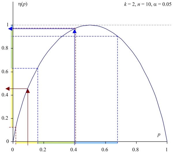
By examination of the maximum, we can define η(p) ∈ (η^–, η⁺) where

η^– = min(η(w^–), η(w⁺)),

η⁺ = (7){ η(w⁺)
η(w^–)
1 if w⁺ < 0.5
if w^– > 0.5
otherwise.

If the interval for p includes the maximum, 0.5, then the upper bound will be the maximum entropy (i.e. 1), and the lower bound will be the smaller of the two transformed bounds. On the other hand, if the interval maps onto a monotonic section of the curve then we simply apply the transformation function to each term.

We plot these intervals over p in Figure 4. The overall shape may be a little unexpected, with wider intervals, representing a modeled expectation of greater sampling uncertainty, about non-central entropy scores.

The dotted lines plot η(w^–) and η(w⁺) respectively: the lower bound is the minimum of the scores, whereas the upper bound reaches 1 for all points where the interval contains 0.5. Thanks to the small sample size in the model n, this is quite a large range.

Figure 4. Plotting the upper and lower confidence interval bounds for binary entropy obtained by Equation (6). We have a ‘folded’ interval at p = 0.4.

Where the interval includes 1, we might say the range is ‘folded’. A subset of entropy scores within the interval may be obtained twice, from two different values of p.

For example, where p = 0.4, (w^–, w⁺) = (0.1682, 0.6873). See Figure 3, middle. The entropy scores for these point bounds (η(w^–), η(w ⁺)) = (0.6535, 0.8962), but the range includes 1. (0.6535, 1].

Since η(w^–) is the lower score, and the range includes 1, any score for p > 0.5 (i.e. from 0.5 to w⁺) obtains a score already accounted for in the range (w^–, 0.5).

This is an example of loss of information resulting from non-monotonic transformation functions. We can’t do very much about this, as it is a direct result of the function. It is similar to the loss of information resulting from representing multi-dimensional differences as a single effect size score.

The interval is also conservative, in that we have taken the minimum of the two transformed bounds. This is a different point.

With this interval, a second proportion p₂ may exceed w⁺ and still obtain entropy values that fall within the interval. Consider the point p₂ = 0.8, whose entropy, η(p₂) = 0.7219, is within the range (0.6535, 1].

In cases like this, there will be a greater than (1 – α) chance that the population score will fall within the folded interval. See also Confidence intervals on goodness of fit ϕ scores. One might use a search procedure to find the optimum point where the error were corrected, by adjusting the α error parameter in the WilsonLower or WilsonUpper function.

Such a step is legitimate, but it would mean that an entropy difference test will necessarily deviate in performance from the standard Binomial model.

We plot the pdf distribution of the unconstrained interval bounds (the ‘I’-shaped error bars in Figure 4) in Animation 1 below. Since entropy scores reverse for p > 0.5 we have not included these. It should be obvious that the distribution of uncertainty is not Normal! This plot also nicely visualises the ‘folding’ phenomenon at η = 1.

Animation 1. Probability density function distributions for p = 0.0 to 0.5. The x-axis is entropy η. The dotted lines are the distributions for the continuity-corrected interval.

Multinomial: Generalised approximations for k > 2

For k > 2 we use the formula for intervals for k-constrained sums (Wallis forthcoming).

In Equation (4) the ‘ln(k)’ term can be treated as a scale constant. Alternatively, one may simply employ log to the base k in the sum.

Let us define the inner term in the sum as inf(p_i) for each term i = 1… k.

inf(p_i) = –p_i.log_k(p_i). (8)

We set inf(p_i) to zero if p_i is 0 or 1. This function is also non-monotonic over the range p_i ∈ [0, 1]. Although both p_i and ln(p_i) are monotonic, the product of two monotonic functions is non-monotonic if one is increasing and the other decreasing.

Next, we need to determine the maximum of the function inf(p_i). This is the same value irrespective of k (recall that ln(k) was a scale factor in Equation (4)). It turns out that the maximum of Equation (7) is where p_i = mˆ = 1/e ≈ 0.367879 (e is Euler’s constant). This has a maximum score, inf(mˆ) ≈ 0.530738.

For each term in the sum, we compute an interval by testing if mˆ is within the interval for p_i.

Let us define an interval inf(p_i) ∈ (h_i^–, h_i⁺), where

h_i^– = min(inf(w_i^–), inf(w_i⁺)),

h_i⁺ = (9){ inf(w_i⁺)
inf(w_i^–)
inf(mˆ)  if w_i⁺ < mˆ
if w_i^– > mˆ
otherwise.

We can plot inf(p_i) and the resulting interval, which we do in Figure 5. The plot is similar to Figure 4, although with a different maximum score, and an eccentric cross-over point close to mˆ.

Figure 5. Plotting the function term inf(p) and transformed intervals, peaking at inf(mˆ). The cross-over point (peak of h^–) is not quite at mˆ.

We compute interval widths for the k-constrained sum by

u^– = √κ Σ(inf(p_i) – h_i^–)², and u⁺ = √κ Σ(inf(p_i) – h_i⁺)², (10)

where kappa κ = k/(k – 1). The resulting interval is simply

η ∈ (η – u^–, η + u⁺). (11)

Using this approximation we can obtain intervals for k = 2 and compare the results directly. See Figure 6.

Figure 6. Comparing the performance of the k-constrained method (Equations (9) and (10)) with the Binomial method of direct transformation (Equation (6)) where k = 2. Note that the k-constrained method is slightly conservative at extremes, but the main penalty is in the middle region. The equivalent Wilson interval is included for comparison. See below.

We saw that the maximum interval for inf(p) exceeded 0.5 for a substantial part of the range, so it is unsurprising to see that the upper interval may overshoot. We can correct for this simply by constraining the interval to η ∈ [0, 1], and it is unlikely to be a problem in practice.

It is rather more important to pay attention to the areas where the interval is within the allowable range but more conservative than that obtained by the direct method, notably in the region near 0.5 (from mˆ to 1 – mˆ). This is clearly a result of averaging the slopes between asymmetric peaks of inf(p) and inf(1 – p).

In a research context, we can accept a more conservative but flexible interval method. Even with rounding errors, the interval will tend to be wider than that obtained by direct calculation.

Comparison with Wilson intervals

How does this interval perform compared to a standard error or Wilson approach? Well, a standard error model of variance about observed values is incorrect. But a Wilson-based model is legitimate in p-space. In Figure 6 we also plotted an interval labelled ‘naïve Wilson interval’, which substitutes η for p into the Wilson score interval (Equation (3)).

We know this approach is naïve and incorrect, but what is the scale of the errors produced?

Our derived entropy intervals are much more conservative (aside from the lower bound ‘peak’). However, the main problem is that the scale of conservatism is different on either side of η. In simple terms, the upper bound is approximately 1/2 the correct width, but the lower bound is too small by 1/√2. The following curves are close to our computed scores, and converge with increased n.

w^– = WilsonLower(η, n/2, α/2),
w⁺ = WilsonUpper(η, n/4, α/2).

An unequal error is a problem for anyone using a naïve variance-based line or model fitting of entropy scores, for the obvious reason that whenever we draw a line through a set of points, we cannot know which side of the ideal line a datapoint will fall on!

Larger n

Returning to our two competing calculation methods, if you experiment with higher values of n in this spreadsheet, you will see that they obtain a smaller area of discrepancy, but this still represents an identifiable loss of sensitivity. However the difference is rather less dramatic than with the pictured n = 10 (which is a very small sample size for estimating entropy, especially with larger k).

Figure 7. The discrepancy between the two calculation methods reduces with larger samples but it does not completely disappear. In all cases the k-constrained method is more conservative.

For small k, combinatorial maths indicates this middle region is liable to be far more likely to occur in practice, so it is worth considering whether this loss is better avoided by substituting the comparison of Multinomial entropy scores with a series of Binomial evaluations, which would also be more straightforward to interpret. On the other hand, if no single observed proportion dominates and exceeds mˆ = 1/e, the method will not lose much power (it will also perform acceptably if it dominates and exceeds 1 – mˆ).

Larger k

Visualising the performance of intervals with higher levels of dimensionality is quite difficult!

To picture the performance of this interval formula with k = 3 terms, the following animation may be helpful. The upper bound becomes convex when p₃ > mˆ. Note that the horizontal axis represents the remaining space, 1 – p₃.

Animation 2. Entropy intervals for k = 3, n = 10 and α = 0.05, permuting values of p₃ from 0.0 to 0.9. The horizontal axis is p₁, and p₂ = p₃ – p₁.

This performance is driven by the shape of the ‘inf’ function (Equation (7)) and its interval (8). See Figure 4.

In brief, when p₃ = 0, the full range of the horizontal axis in Figure 4 (from 0 to 1) is available to p₁ (and p₂), and inf(p₃) = 0. This obtains a set of curves similar to Figure 5, but adjusted by the 95% interval for inf(p₃) ∈ (h₃^–, h₃⁺) = (0, 0.3238).

As p₃ increases, the available range reduces, so that when p₃ = 0.3, say, p₁ ranges from 0 to 0.7. inf(p₃) = 0.3288 with interval (0.2186, 0.3349), and the curve is generated by ‘inf’ functions for p₁ and p₂ over the remaining range.

Where p₃ = 1, p₁ = p₂ = 0, so η = 0, with a 95% confidence interval (0, 0.6190).

As before, note we are using a rather unrealistically small sample size, n = 10, with three outcomes, hence the wide interval. This is useful to expose any unusual behaviour of functions and to confirm to us the method is robust, but few studies will rely on such small samples. Indeed, one would generally assume that n >> k.

Conclusions

We have demonstrated how to obtain confidence intervals for information and entropy estimates obtained from samples. The interval for an observed information score is a monotonic transformation of a Binomial interval for the simple proportion.

How do we test if two information scores are significantly different? Since ι(p) is a monotonic function of p, we can employ a contingency table and test (Fisher, 2 × 2 χ² or Newcombe-Wilson). If the test is significant, the scores must differ.

We derived two methods of computation for entropy confidence intervals, one for simple Binomial alternatives, where k = 2, and a more general approximation for Multinomial outcomes. Provided that proportions {p_i} are properly Multinomial (and therefore free to vary), the Binomial approximation and k-constrained sum are appropriate. The latter is more conservative than the method of direct transformation for k = 2, so in these cases the Binomial method is preferable.

Armed with interval methods, we can also employ Zou and Donner’s (2008) difference theorem for comparing the significant difference between any two independently observed properties. See Wallis (forthcoming) and An algebra of intervals.

These methods are robust and, since they are based on the Wilson score interval, they are also capable of accepting a continuity correction and other types of sampling adjustment. We plot the continuity-corrected interval for information scores by way of example: we could do likewise for entropy, however in this blog post it is more important to focus on the difference between alternative methods of computation. Nonetheless whenever we refer to the Wilson score interval we are really referring to a class of configurable methods.

References

Kumar, U., V. Kumar and J.N. Kapur (1986). Normalised measures of entropy. International Journal of General Systems 12:1, 55-69.

Shannon, C. E. and W. Weaver (1949). The Mathematical Theory of Communication. Urbana, Illinois: University of Illinois Press, 1949.

Wallis, S.A. (2013). Binomial confidence intervals and contingency tests: mathematical fundamentals and the evaluation of alternative methods. Journal of Quantitative Linguistics 20:3, 178-208. » Post

Wallis, S.A. (2021). Statistics in Corpus Linguistics Research. New York: Routledge. » Announcement

Wallis, S.A. (forthcoming). Accurate confidence intervals on Binomial proportions, functions of proportions and other related scores. » Post

Wilson, E.B. 1927. Probable inference, the law of succession, and statistical inference. Journal of the American Statistical Association 22: 209-212.

Zou, G.Y. & A. Donner (2008). Construction of confidence limits about effect measures: A general approach. Statistics in Medicine, 27:10, 1693-1702.

See also

• Excel spreadsheet
• An algebra of intervals
• Plotting entropy confidence interval distributions
• Confidence intervals on goodness of fit ϕ scores
• The confidence of diversity
• Correcting for continuity