Introduction
Inferential statistics is a methodology of extrapolation from data. It rests on a mathematical model which allows us to predict values in the population based on observations in a sample drawn from that population.
Central to this methodology is the idea of reporting not just the observation itself but also the certainty of that observation. In some cases we can observe the population directly and make statements about it.
- We can cite the 10 most frequent words in Shakespeare’s First Folio with complete certainty (allowing for spelling variations). Such statements would simply be facts.
- Similarly, we could take a corpus like ICE-GB and report that in it, there are 14,275 adverbs ending in -ly out of 1,061,263 words.
Provided that we limit the scope of our remarks to the corpus itself, we do not need to worry about degrees of certainty because these statements are simply facts. Statements about the corpus are sometimes called descriptive statistics (the word statistic here being used in its most general sense, i.e. a number).
From description to inference
However in many cases we wish to generalise from a sample to unseen data. Indeed experimental research is not motivated by simply describing the outcome of the experiment but predicting the likely implications of our results.
- We could hypothesise that the First Folio is, in some respect, “representative” of
- all of Shakespeare’s plays,
- the writing of Elizabethan English playwrights, or
- Early Modern English.
If we want to generalise from the First Folio to any of the above, we need to make inferential hypotheses.
I have used the term “representative” here to mean “an accurate predictor of”. So we might hypothesise (predict) that the top 10 words in the First Folio were the same top 10 words in Shakespeare’s published plays, in the plays of his contemporaries or indeed EModE more generally.
This thought experiment illustrates an important principle. Even if we know nothing else about the sample, the less similar the population is from our sample (either because it is not a random subset or because it must be a tiny subset), the more likely it is that the sample is unrepresentative of the population – and the weaker the inference can be.
The standard inferential statistical model assumes that the population is much larger than the sample and the sample is a genuine random sample (drawn from the population) of the term in question. However, optimal methods for obtaining a random subset of cases in the population is a complex question when we are dealing with samples drawn from a finite number of pieces of running text.
Note: Below we note that there is a continuum between a finite population (e.g. describing the First Folio itself) and a random sample drawn from an infinite or very large population (all of EModE). It is possible to make improved estimates of certainty for samples which are a substantive subset of the population.
As we have seen, inferential statistics is central to experimental research. Research requires us to make predictions from our results to the overall population. If we were to repeat our experiment we could resample the population and obtain different results. The question then is how different are results likely to be. We incorporate this uncertainty into statements by calculating confidence intervals or performing statistical tests.
Inferential statements are also expected to be robust. Consequently when I refer to “statistics” on this blog, I mean inferential statistics, unless otherwise stated. Descriptive statistics merely describe what you can see in your results, not what you are likely to see were you to repeat the experiment.
The key inferential concept: confidence intervals
The standard deviation for an expected, or population probability, P, can be computed simply using a method termed “the Normal approximation to the Binomial”. The Binomial model is a mathematical model of simple chance. After a number of assumptions are made (samples are random, values are free to vary, etc), we can write:
Standard deviation S ≡ √P(1 – P)/n.
This standard deviation is a measure of the expected spread of observations about a given P. This is not always very useful, however, because when we are plotting data, we often have lots of observed probabilities, which we will denote as p, but we don’t actually know what the ‘true’ value, P, is!
Therefore the most useful starting point for inferential statistics is a confidence interval. A confidence interval is drawn around the observation, p. It gives us a range of values around p where P is likely to be found.
Significance tests are derived from confidence intervals (Wallis 2013). To plot accurate intervals around observed p we need to calculate Wilson’s score interval:
Wilson score interval (w–, w+) ≡ p + z²/2n ± z√p(1 – p)/n + z²/4n²
1 + z²/n.
The constant z is the two-tailed critical value of the standard Normal distribution at a given error level α (e.g., 0.05), usually spelled out as zα/2.
We can also attach interval bounds to Wilson functions like this:
w– = WilsonLower(p, n, α/2), and w+ = WilsonUpper(p, n, α/2).
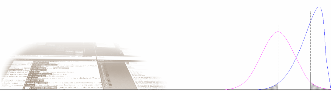
This formula assumes that the population is infinite – or much larger than the sample at least (see the figure below, right).
Q. What happens if the sample is the population?
A. The observation would be certain – and the interval width e must fall to zero (below, left).

When samples become populations (or large parts of them)
If the population is finite and the sample approaches the population in size (e.g. if the First Folio was treated as a sample of Shakespeare’s published plays) then the degree of uncertainty associated with the prediction (the standard deviation) decreases in size. The idea is summarised in the figure above.
According to Singleton et al. (1988), the scale of this decline is approximately in proportion to ν = √1 – n/N, where n is the size of the sample and N the size of the population. Recent sources use the following equation, which obtains a very similar value:
Finite population adjustment ν = √(N – n)/(N – 1).
Note: the only difference between the two equations is the denominator (population size N) differs by 1.
This factor can be multiplied by the standard deviation, to obtain a smaller confidence interval:
Corrected standard deviation S ≡ ν√P(1 – P)/n.
This adjustment divides n by ν², so it may also be applied to the Wilson score interval. The easiest way to do this is with Wilson functions:
w– = WilsonLower(p, n/ν², α/2), and w+ = WilsonUpper(p, n/ν², α/2).
Since ν is less than 1, dividing n by ν² causes the width of the interval to decrease and the adjusted centre to tend towards p. See this Wilson sample-population interval calculator for the calculation.
This adjustment is also used when calculating error intervals on subsamples. In this case, the ‘population’ is the initial finite sample. See Coping with imperfect data for an example.
Computational statistics
The distinction between descriptive and inferential statistics has become rather confused by a third development. This is the rise of computation.
Since algorithms may be extremely complex, it can be difficult for a lay reader to determine whether such “computational statistics” are really inferential statistics (and therefore citable in experimental results) or just descriptive statistics, albeit of a particularly sophisticated variety.
Computer processes can be applied to either descriptive statistics (much information theoretic modelling is of this nature) or inferential statistics (e.g. log-linear modelling, or logistic regression).
The fact of computation does not tell us whether or not the computation is essentially descriptive or inferential. In order to do this we ask the following question:
- how does the computation address the uncertainty of input data (observations)?
For example, part-of-speech taggers are algorithms which obtain probabilities, termed transition probabilities or marginal probabilities, referring to the likelihood that word class B follows word class A. These probabilities are computed from data descriptively, i.e. without considering the certainty of the probability estimate itself. So, strictly speaking, the database of a POS-tagger contains descriptive statistics, although the tagger is usually employed on new data.
The reason why POS-taggers perform with high (95%+) accuracy on novel data is most likely due to stable properties of language (constraint, or lack of freedom to vary on many word class tags) and because the observation is supported by enough data, rather than because they model uncertainty (they don’t).
Descriptive statistics can be extremely useful, and in many cases it may not be possible to factor in the certainty of an observation as well as the observation itself.
Exploratory statistics
Perhaps one of the most useful kinds of statistical and quasi-statistical approaches involves visualising distributions by plotting graphs of various kinds.
Like computational statistics, exploratory statistics (or exploratory data analysis, EDA) is not really a class of statistics. It is a healthy method for exploring unknown data which draws on both descriptive and inferential statistics.
Graph plotting is extremely powerful because you can immediately see if data is conforming to an expected pattern. This is also an area where computer technology has made the job of the analyst much easier. Whether one uses R or Excel to plot graphs, the importance of actually plotting your data cannot be underestimated.
Exploratory analysis can lead to real discoveries, provided you are prepared to experiment. Note that as with any other method, when we plot and interpret graphs we make assumptions about our data.
Perhaps the best way of illustrating this is with a real example, cited in Wallis (2019). I’ll try to take you through the steps I went through.
Step 1. Some data
Consider the following data from ICE-GB. Note that the values in the bottom row, marked “at least x”, are the cumulative frequency, F(x), of the figures above (155 = 148+7, 2,944 = 2,789+148+7, etc.).
Initially I was not sure whether I needed exact frequency f(x), or cumulative frequency F(x). In fact the method used for data retrieval, ICECUP’s Fuzzy Tree Fragments, tends to make the retrieval of general patterns (an NP with at least this number of AJPs before the Head) easier and more natural than those requiring an exact match (precisely this number of AJPs in an NP).
Another way of thinking about this data is that there are, in total, 193,195 NPs with common noun heads in ICE-GB, and around 20% of these (37,305) contain an attributive adjective phrase. The probability of a speaker choosing to add an adjective phrase to an NP without one is therefore around 0.2.
A similar calculation can be performed between subsequent pairs of cumulative frequencies. This will become useful later on, as we shall see.
| number of AJPs x | 0 | 1 | 2 | 3 | 4 |
| f(x) exactly x | 155,830 | 34,361 | 2,789 | 148 | 7 |
| F(x) at least x | 193,195 | 37,305 | 2,944 | 155 | 7 |
Distribution of the number of attributive adjective phrases in common noun-headed NPs in ICE-GB. Upper row: simple frequency distribution f(x), lower: cumulative frequency distribution F(x).
Step 2. An initial exploration
The first step was simply to plot the cumulative frequency distribution. This obtains the following graph.

This looks very much like a well-known mathematical series called an exponential decay curve (or, more correctly, the “geometric distribution”). This distribution is what you would expect if every decision to add an AJP was independent from the previous one, like tossing a series of unbiased coins (½, ¼, ⅛, ¹/16, etc.).
The ‘quick and dirty’ way of checking whether data matches this pattern is to change the y axis from a linear scale, F(x), to a logarithmic scale, log(F(x)). A straight line indicates that the data conforms to an exponential distribution.
This is what I got.

This is interesting, because the graph is not a straight line. It is almost a straight line, but crucially it appears to bend downwards.
We have a lot of data so it seems likely that the pattern is statistically significant (I had not considered which tests would be applicable at this point). Something must be going on.
Step 3. Rethinking the data
The next stage was to work out how we could reformat the data a third way to reveal this pattern and possibly test for significance.
The solution was to go back to our coin-tossing example. When you toss a coin, each throw is independent from the previous one. Even if the coin were biased, so that the probability of a head was not 0.5 but 0.8 (say), the fact that the previous toss had obtained a head would not affect the next one.
The probability would be constant. So the key question is as follows:
Is the probability of adding an attributive AJP in our data constant, or is it affected by the previous additions (throws)?
The way to find out is to plot the probability distribution p(x) = F(x) / F(x – 1).

Step 4. Testing for significance
Note that at this point we can also now move from descriptive statements to inferential statements by introducing confidence intervals.
We plot Wilson score intervals on each probability and test for significance with a goodness-of-fit test. This is justified by the fact that we are observing data in serial subset relationships, so the data supporting p(2) is a subset of the data supporting p(1), and so on.
This test is applied at each step to compare each Wilson interval bound with its preceding observed probability (arrowed). This is isometric to employing the single-sample z test for the preceding probability, or a goodness-of-fit χ² test rather than a 2 × 2 test.
The data can be laid out as below.
| number of AJPs x | 0 | 1 | 2 | 3 | 4 |
| f(x) exactly x | 155,830 | 34,361 | 2,789 | 148 | 7 |
| F(x) at least x | 193,195 | 37,305 | 2,944 | 155 | 7 |
| p(x) probability | 0.1932 | 0.0789 | 0.0526 | 0.0452 | |
| w+(x) upper | |||||
| w–(x) lower | 0.0762 | 0.0451 | 0.0220 |
Complete table with probability p(x) and bounds of the 95% Wilson score interval. To test for a significant fall (bold), compare w+(x) < p(x – 1).
Since, far from being constant, the probability falls with each successive addition, we can say that the addition of attributive adjective phrases to NPs with common noun heads becomes more difficult as the NP becomes longer.
The unconscious decisions that speakers/writers make to add an AJP to a noun phrase are not independent, but interact in a retarding, negative feedback loop of some kind.
The point of this example is to show how research is often a process of discovery, and that you may need to reformat or re-present your data to reveal patterns or test results.
In particular, in significance testing you need to understand the underlying model to identify what the null hypothesis should be: in our case, that cumulative frequency followed a geometric distribution and therefore the probability of addition was constant. Overturning that null hypothesis allowed us to demonstrate a new result.
The task would then be to explain this result… See Wallis (2019) for what I think this study reveals.
Some brief recommendations
- In experiments, when reporting results we should always cite inferential statistics where possible. Statistical tests may be possible if you can rethink your data appropriately.
- Descriptive statistical methods should be specifically noted as such, and cited only when there is no other available inferential method (including a less powerful test or one with a theoretically weaker conclusion).
- Finally, if an inferential statistical test does not obtain a significant result, the result is not “indicative” but non-significant!
References
Singleton, R. Jr., B.C. Straits, M.M. Straits and R.J. McAllister, 1988. Approaches to social research. New York, Oxford: OUP.
Wallis, S.A. 2013. z-squared: the origin and application of χ². Journal of Quantitative Linguistics 20:4, 350-378. » Post
Wallis, S.A. 2019. Investigating the additive probability of repeated language production decisions. International Journal of Corpus Linguistics 24:4, 490-521. » Post
