Confidence intervals for Cohen’s h

1. Introduction

Cohen’s h (Cohen, 2013) is an effect size for the difference of two independent proportions that is sometimes cited in the literature. h ranges between minus and plus pi, i.e. h ∈ [–π, π].

Jacob Cohen suggests that if |h| > 0.2, this is a ‘small effect size’, if |h| > 0.5, it is ‘medium’, and if |h| > 0.8 it is ‘large’. This conventional application of effect sizes – as a descriptive method for distinguishing sizes – is widespread.

The score is defined as the difference between the arcsine transform of the root of Binomial proportions pi for i ∈ {1, 2}, hence the expanded range, ±π.

That is,

h = ψ(p1) – ψ(p2),(1)

where the transform function ψ(p) is defined as

ψ(p) = 2 arcsin(√p).(2)

In this blog post I will explain how to derive an accurate confidence interval for this property h. The benefits of doing so are multiple.

  1. We can plot h scores with intervals, so we can visualise the reliability of their estimate, pay attention to the smallest bound, etc.
  2. We can compare two scores, h1 and h2, for significant difference. In other words, we can conclude that h2 > h1, or vice versa.
  3. We can reinterpret ‘large’ and ‘small’ effects for statistical power.
  4. We can consider whether an inner bound is greater than Jacob’s thresholds. Thus if h is positive, if h > 0.5 we can report that the likely population score is at least a ‘medium’ effect.

An absolute (unsigned and non-directional) version of |h| is sometimes cited. We can compute intervals for unsigned |h|. We will return to this question later.

Continue reading “Confidence intervals for Cohen’s h”

Confidence intervals

In this blog we identify efficient methods for computing confidence intervals for many properties.

When we observe any measure from sampled data, we do so in order to estimate the most likely value in the population of data – ‘the real world’, as it were – from which our data was sampled. This is subject to a small number of assumptions (the sample is randomly drawn without bias, for example). But this observed value is merely the best estimate we have, on the information available. Were we to repeat our experiment, sample new data and remeasure the property, we would probably obtain a different result.

A confidence interval is the range of values in which we predict that the true value in the population will likely be, based on our observed best estimate and other properties of the sample, subject to a certain acceptable level of error, say, 5% or 1%.

A confidence interval is like a blur in a photograph. We know where a feature of an object is, but it may be blurry. With more data, better lenses, a greater focus and longer exposure times, the blur reduces.

In order to make the reader’s task a little easier, I have summarised the main methods for calculating confidence intervals here. If the property you are interested in is not explicitly listed here, it may be found in other linked posts.

1. Binomial proportion p

The following methods for obtaining the confidence interval for a Binomial proportion have high performance.

  • The Clopper-Pearson interval
  • The Wilson score interval
  • The Wilson score interval with continuity correction

A Binomial proportion, p ∈ [0, 1], and represents the proportion of instances of a particular type of linguistic event, which we might call A, in a random sample of interchangeable events of either A or B. In corpus linguistics this means we need to be confident (as far as it is possible) that all instances of an event in our sample can genuinely alternate (all cases of A may be B and vice-versa).

These confidence intervals express the range of values where a possible population value, P, is not significantly different from the observed value p at a given error level α. This means that they are a visual manifestation of a simple significance test, where all points beyond the interval are considered significantly different from the observed value p. The difference between the intervals is due to the significance test they are derived from (respectively: Binomial test, Normal z test, z test with continuity correction).

As well as my book, Wallis (2021), a good place to start reading is Wallis (2013), Binomial confidence intervals and contingency tests.

The ‘exact’ Clopper-Pearson interval is obtained by a search procedure from the Binomial distribution. As a result, it is not easily generalised to larger sample sizes. Usually a better option is to employ the Wilson score interval (Wilson 1927), which inverts the Normal approximation to the Binomial and can be calculated by a formula. This interval may also accept a continuity correction and other adjustments for properties of the sample.

Continue reading “Confidence intervals”

Plotting entropy confidence interval distributions

Introduction

In this blog post, I will discuss the distribution of confidence intervals for the information-theoretic measure, entropy.

One of the problems we face when reasoning with statistical uncertainty concerns our ability to mentally picture its shape. As students we were shown the Normal distribution and led to believe that it is reasonable to assume that uncertainty about an observation is Normally distributed.

Even when students are introduced to other distributions, such as the Poisson, the tendency to assume that uncertainty is expressed as a Normal distribution (‘the Normal fallacy’) is extremely common. The assumption is not merely an issue of weak mathematics and poor conceptualisation: since Gauss’s famous method of least squares relies on Normality, this issue affects fitting algorithms and error estimation applied to non Real variables, such as the one discussed here.

As a general rule, whenever I have developed methods for computing confidence intervals I have done my best to plot, not just the interval bounds (the upper or lower critical threshold at a given error level) but the probability density function (pdf) distribution of the interval bounds. The results are often surprising, and gain us fresh insight into the intervals we are using.

Entropy is an interesting case study for two reasons. First, there are two methods for computing the two-valued measure, one more precise but less generalisable than the other. Second, like many effect sizes, the function involves a non-monotonic transformation, which has important implications for how we conceptualise uncertainty and intervals. (Indeed, so far I have not published the equivalent distributions for goodness of fit ϕ or diversity, both of which engage the same type of transformations.)

First we will do some necessary recapitulation, so bear with me. Continue reading “Plotting entropy confidence interval distributions”