The confidence of diversity

Introduction

Occasionally it is useful to cite measures other than simple proportions (probabilities of selection) or differences in probability. When we do, we should estimate confidence intervals on these measures. There are a number of ways of estimating intervals, including bootstrapping and simulation, but these are computationally heavy.

For many measures it is possible to derive intervals from the Wilson score interval by employing a little mathematics. Elsewhere in this blog I discuss how to manipulate the Wilson score interval for simple transformations of p, such as 1/p, 1 – p, etc. In An algebra of intervals we discuss algebraic combinations of independent properties.

Below I am going to explain how to derive an interval for grammatical diversity, d, which we can define as the probability that two randomly-selected instances have different outcome classes.

Diversity is an effect size measure of a frequency distribution, i.e. a vector of k frequencies. If all frequencies are the same, the data is evenly spread, and the score will tend to a maximum. If all frequencies except one are zero, the chance of picking two different instances will of course be zero. Diversity is well-behaved except where categories have frequencies of 1.

To compute this diversity measure, we sum across the set of outcomes (all functions, all nouns, etc.), C:

diversity d = ∑ p₁(c).(1 – p₂(c)) if n > 1; 1 otherwise,(1)

where c ∈ C and C is a set of k > 1 disjoint categories, p₁(c) is the probability that item 1 is category c and p₂(c) is the probability that item 2 is the same category c.

We have observed probabilities

p₁(c) = o(c)/n,
p₂(c) = (o(c) – 1)/(n – 1) = (p₁(c).n – 1)/(n – 1),(2)

where o(c) is the observed frequency for type c and n is the total number of instances.

The formula for p₂ includes an adjustment for the fact that we already know that the first item is c. This principle is used in card-playing statistics. Suppose I draw cards from a pack. If the first card I pick is a heart, I know that there are only 10 other hearts in the pack, so the probability of the next card I pick up being a heart is 10 out of 51, not 11 out of 52.

Note that as the set is closed, ∑p₁(c) = ∑p₂(c) = 1.

The maximum score is slightly less than (k – 1) / k except in the special case where n approaches k and there is a frequency of 1 in any category, in which case diversity can approach 1.

An example

In a paper with Bas Aarts and Jill Bowie (2018), we found that the share of functions of –ing clauses (‘gerunds’) appeared to change over time in the Diachronic Corpus of Present-day Spoken English (DCPSE).

We obtained the following graph. The bars marked ‘LLC’ refer to data drawn from the period 1956-1972; those marked ‘ICE-GB’ are from 1990-1992.

Figure 1. Changes in proportion of p(function | –ing) between LLC (1960s-70s) and ICE-GB (1990s) data in DCPSE, ordered by total frequency. After Aarts et al. (2018).

This graph considers six functions C = {CO, CS, OD, SU, A, PC} of the clause. It plots p(c) over c. Considered individually, some functions significantly increase and some decrease their share. Note also that the increases appear to be concentrated in the shorter bars (smaller p) and the decreases in the longer ones.

Intuitively this appears to mean that we are seeing –ing clauses increase in their diversity of grammatical function over time. We would like to test this proposition.

Here is the observed LLC frequency data, o(c).

CO	CS	SU	OD	A	PC	Total
6	33	61	326	610	1,203	2,239

Table 1. LLC frequency data: a simple array of k values. Diversity is computed out of the proportions occupied by each one, in this case, p(function | –ing).

Computing diversity scores, we arrive at

d(LLC) = 0.6152 and d(ICE-GB) = 0.6443.

Confidence intervals for d

We wish to compare these two diversity measures. The first step is to estimate a confidence interval for d.

Step 1: intervals for each term

First we compute interval estimates for each term, d(c) = p₁(c).(1 – p₂(c)). We employ the Wilson score interval for a probability p, which we will denote by (w^–, w⁺). For reference, this is written as

Wilson score interval (w^–, w⁺) ≡ p + z²/2n ± z√p(1 – p)/n + z²/4n²
1 + z²/n,
(3)

where z is the critical value of the two-tailed Normal distribution at error level α, properly written z_α/2. A continuity correction, to compensate for the discrete nature of the Binomial, may also be employed.

Any monotonic function of p, fn(p), can be applied and plotted as a simple transformation. See Reciprocating the Wilson interval. We can write

fn(p) ∈ (fn(w^–), fn(w⁺)).

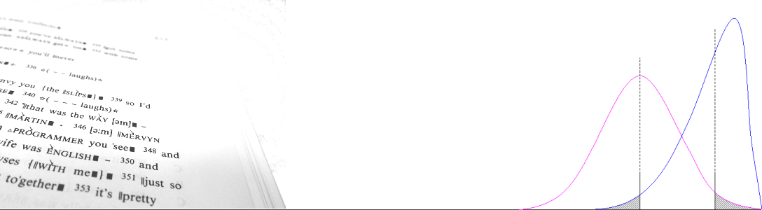
However, d(c) is not monotonic over its entire range. Indeed d(c) reaches a maximum where p = 0.5. However the axiom holds conservatively provided that the function is monotonic across the interval (w^–, w⁺), i.e. where 0.5 is not within the interval. The following graph plots d(c) over p(c) for a two-cell vector where n = 40.

Figure 2. Diversity vs. probability for each cell in a 2-cell vector. Diversity is globally non-monotonic, peaking at p = 0.5, but locally monotonic.

We can rewrite each term in Equation (1), d(c), in terms of a probability p and n,

d(p, n) = p × (1 – (p × n – 1) / (n – 1)).(4)

This has the interval

d(p, n) ∈ (d(w^–, n), d(w⁺, n))

provided that d(w⁺, n) < 0.5. To obtain the interval we have simply plugged w^– and w⁺ into the formula for d(p, n) in place of p. It is worth noting that Equation (4) approximates to p(1 – p).

Indeed, noting the shape of d, we can derive the following.

d(p, n) ∈ (d(w^–, n), d(w⁺, n)) where w⁺ < 0.5,
d(p, n) ∈ (d(w⁺, n), d(w^–, n)) where w^– > 0.5,
d(p, n) ∈ (min(d(w^–, n), d(w⁺, n)), d(0.5, n)) otherwise.

Figure 3. Where the interval includes the maximum of d, the upper bound will be this maximum value.

Elsewhere we discuss the fact that an interval with a turning point in it like this ‘folds’ the bounds on top of each other, making the bound falling within the interval conservative. However, for now we will simply accept this additional conservatism.

Step 2: summation of terms

Next we need to sum these intervals. To do this we need to take account of the number of degrees of freedom of the vector.

The Bienaymé theorem states that the variance of a set of independent terms is the sum of the independent variances.

variance s² = ∑s_i².(5)

Newcombe (1998) and Zou and Donner (2008) estimate variance by summing the squared interval widths of k independent terms (see also An algebra of intervals). The assumption is that the independent sum of standard deviations is the hypotenuse of a triangle whose standard deviations are tangential.

l = √∑[d(p(c), n) – d(w^– (c), n)]², and
u = √∑[d(p(c), n) – d(w⁺ (c), n)]².(6)

A sum of k independent Normally distributed terms has k degrees of freedom. But in a conventional ‘goodness of fit’ condition the total variance has k – 1, rather than k, degrees of freedom. We propose a ‘k-constrained Bienaymé theorem’ in the form:

constrained var. s′² = κ∑s_i².(7)

In the case of χ², κ = k/(k – 1) converges to the equivalent dependent single Wilson interval when k = 2.

When df = 2, the terms d(p(1), n) and d(p(2), n) are deterministically related to each other because p(1) + p(2) = 1. In Equation (1), each term approximates to the same value p(1) × p(2). In chi-square the equivalent terms are p(1) and p(2), s₁ = s₂ and Equation (7) becomes 4s_i², and s′ = 2s_i i.e., two standard deviations.

This obtains κ = 2 when k = 2 (approximating to the simple summation) and κ → 1 as k → ∞ (an independent sequence).

We may use this principle to construct a k-constrained interval.

l′ = √κ∑[d(p(c), n) – d(w^– (c), n)]², and
u′ = √κ∑[d(p(c), n) – d(w⁺ (c), n)]²,(8)

where κ is the appropriate adjustment. 

Example data

To see how this works, let’s return to our example. The following is drawn from the LLC data (first, blue bar in the graph), at an error level α = 0.05. Here is the data for each simple proportion and the Wilson score interval at α = 0.05.

function	CO	CS	SU	OD	A	PC
p	0.0027	0.0147	0.0272	0.1456	0.2724	0.5373
w–	0.0012	0.0105	0.0213	0.1316	0.2544	0.5166
w+	0.0058	0.0206	0.0348	0.1608	0.2913	0.5579

Table 2. Proportions and 95% Wilson interval for the LLC frequency data.

Next we apply Equation (4) to w^– and w⁺. Here is the resulting data for d(p, n) and its lower bound. Note that one of our cells (PC) has p₁ > 0.5, w₁^– is also > 0.5, so we swap the interval bounds obtained (0.2498, 0.2468).

function	CO	CS	SU	OD	A	PC
d(p, n)	0.0027	0.0145	0.0265	0.1245	0.1983	0.2487
p1 = w–	0.0012	0.0105	0.0213	0.1316	0.2544	0.5166
p2	0.0008	0.0101	0.0208	0.1312	0.2541	0.5164
d(w–, n)	0.0012	0.0104	0.0208	0.1143	0.1898	0.2468

Table 3. Computing d(p, n) and the lower bound of each term, d(w^–, n).

The resulting inner lower width for d, l, is summed using Equation (8) with κ = 8/6 = 1.2, obtaining l = 0.017539 (to six decimal places). We repeat the summation for the upper bound.

l′ = √κ∑[d(p(c), n) – d(w^– (c), n)]² = 0.0166,
u′ = √κ∑[d(p(c), n) – d(w⁺ (c), n)]² = 0.0181.

This obtains a final interval of (0.5986, 0.6333) without continuity correction.

By this method we can quote diversity for LLC and ICE-GB with absolute intervals (d – l, d + u):

d(LLC) = 0.6152 ∈ (0.5986, 0.6333), and
d(ICE-GB) = 0.6443 ∈ (0.6256, 0.6644).

Testing for differences in diversity

In the Newcombe-Wilson test, we compare the difference between two Binomial observations p₁ and p₂ with the Pythagorean distance of the Wilson interval widths u₁ = w₁⁺ – p₁, etc. This can be written as

–√u₁ ² + l₂ ² < (p₁ – p₂) < √l₁ ² + u₂ ².

If the equation above is true, the result is not significant. The difference falls within the zero-based confidence interval on the distance.

This method operates on the assumption that the observations are independent and variances are approximately Normal. Indeed, the latter assumption may be relaxed. Zou and Donner (2008) argue that good interval coverage is sufficient. By analogy we can employ l′₁ and u′₁, etc. to test difference intervals for diversity:

–√u′₁² + l′₂² < (d₁ – d₂) < √l′₁² + u′₂².(9)

Our observations are drawn from independent samples, the difference in diversity is -0.0291, and the resulting zero-based difference interval is (-0.0260, +0.0261). Since the difference falls outside this interval, we can report that it is significant, and ICE-GB does exhibit significantly greater diversity of outcome than LLC.

Conclusions

In many scientific disciplines, such as medicine, papers that include graphs or cite figures without confidence intervals are considered incomplete and are likely to be rejected by journals. However, whereas the Wilson interval performs admirably for simple Binomial probabilities, computing confidence intervals for more complex measures typically involves a more involved computation.

We defined a diversity measure and derived a confidence interval for it. Although probabilistic (diversity is indeed a probability), it is not a Binomial probability. For one thing, it has a maximum below 1, of slightly in excess of (k – 1) / k. For another, it is computed as the sum of the product of two sets of related probabilities.

In order to derive this interval we started with the assumption of monotonicity, i.e. that a function tends to increase along its range, or decrease along its range. However, for any single cell, d is decidedly not monotonic – it increases as p tends to 0.5 but falls thereafter. We employed the weaker assumption that it is monotonic within the confidence interval, or – in the case where the interval includes a change in direction – that it cannot exceed the global maximum.

We computed an interval by employing a constrained estimate of variance, noting that the vector has k – 1 degrees of freedom. This is sufficient for us to derive an interval, and, by employing Newcombe’s method, a test of significant difference.

Like Cramér’s ϕ, diversity condenses an array with k – 1 degrees of freedom into a variable with a single degree of freedom. Swapping data between the smallest and largest columns would obtain exactly the same diversity score.

Testing for significant difference in diversity, therefore, is distinct from carrying out a k × 2 chi-square test. Such a test could be significant even when diversity scores are not significantly different. Our diversity difference test is more conservative, and significant results may be more worthy of comment.

References

Aarts, B., Wallis, S.A., and Bowie, J. (2018). –Ing clauses in spoken English: structure, usage and recent change. In Seoane, E., C. Acuña-Fariña, & I. Palacios-Martínez (eds.) Subordination in English. Synchronic and Diachronic Perspectives. Topics in English Linguistics (TiEL) 101. Berlin: De Gruyter. 129-154.

Newcombe, R.G. (1998). Interval estimation for the difference between independent proportions: comparison of eleven methods. Statistics in Medicine, 17, 873-890.

Zou, G.Y. & A. Donner (2008). Construction of confidence limits about effect measures: A general approach. Statistics in Medicine, 27:10, 1693-1702.

See also

• Diversity interval example (Excel)
• Is “grammatical diversity” a useful concept?
• An algebra of intervals
• Reciprocating the Wilson interval
• Goodness of fit measures for discrete categorical data
• Measures of association for contingency tables