Introduction Paper (PDF)
Conventional stochastic methods based on the Binomial distribution rely on a standard model of random sampling whereby freely-varying instances of a phenomenon under study can be said to be drawn randomly and independently from an infinite population of instances.
These methods include confidence intervals and contingency tests (including multinomial tests), whether computed by Fisher’s exact method or variants of log-likelihood, χ², or the Wilson score interval (Wallis 2013). These methods are also at the core of others. The Normal approximation to the Binomial allows us to compute a notion of the variance of the distribution, and is to be found in line fitting and other generalisations.
In many empirical disciplines, samples are rarely drawn “randomly” from the population in a literal sense. Medical research tends to sample available volunteers rather than names compulsorily called up from electoral or medical records. However, provided that researchers are aware that their random sample is limited by the sampling method, and draw conclusions accordingly, such limitations are generally considered acceptable. Obtaining consent is occasionally a problematic experimental bias; actually recruiting relevant individuals is a more common problem.
However, in a number of disciplines, including corpus linguistics, samples are not drawn randomly from a population of independent instances, but instead consist of randomly-obtained contiguous subsamples. In corpus linguistics, these subsamples are drawn from coherent passages or transcribed recordings, generically termed ‘texts’. In this sampling regime, whereas any pair of instances in independent subsamples satisfy the independent-sampling requirement, pairs of instances in the same subsample are likely to be co-dependent to some degree.
To take a corpus linguistics example, a pair of grammatical clauses in the same text passage are more likely to share characteristics than a pair of clauses in two entirely independent passages. Similarly, epidemiological research often involves “cluster-based sampling”, whereby each subsample cluster is drawn from a particular location, family nexus, etc. Again, it is more likely that neighbours or family members share a characteristic under study than random individuals.
If the random-sampling assumption is undermined, a number of questions arise.
- Are statistical methods employing this random-sample assumption simply invalid on data of this type, or do they gracefully degrade?
- Do we have to employ very different tests, as some researchers have suggested, or can existing tests be modified in some way?
- Can we measure the degree to which instances drawn from the same subsample are interdependent? This would help us determine both the scale of the problem and arrive at a potential solution to take this interdependence into account.
- Would revised methods only affect the degree of certainty of an observed score (variance, confidence intervals, etc.), or might they also affect the best estimate of the observation itself (proportions or probability scores)?
Excerpt
We will employ a method related to ANOVA and F-tests, applying this method to a probabilistic rather than linear scale. This step is not taken lightly but as we shall see in Section 6, it can be justified.
Consider an observation p drawn from a number of texts, t′, based on n total instances. These must be non-empty texts, i.e. for all i = 1..t′ texts, ni > 0. Were the sample drawn randomly from an infinite population, we could employ the Normal approximation to the Binomial distribution
standard deviation S ≡ √P(1 – P)/n.
variance S² = P(1 – P)/n,(1)
where P is the mean proportion in the population and n the sample size. Inverting the above (so that P = w– when p = P + zα/2.S), we have the Wilson score interval, which may be directly computed by
(2)Wilson interval (w–, w+) ≡ p + zα/2²/2n ± zα/2√p(1 – p)/n + zα/2²/4n²
1 + zα/2²/n,
where zα/2 is the critical value of the Normal distribution for a given error level α (see Wallis 2013 for a detailed discussion). Other derivations from (1) include χ² and log-likelihood tests, least-square line-fitting, and so on.
The model assumes that all n instances are randomly drawn from an infinite (or very large) population. However, we suspect that our subsamples are not equivalent to random samples, and that this sampling method will affect the result.
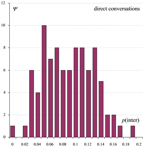
To investigate this question, our approach involves two stages. First, we measure the variance of scores between text subsamples according to two different models, one that presumes that each subsample is a random sample, and one calculated from the actual distribution of subsample scores. Consider the frequency distribution of probability scores, pi, across all t′ non-empty texts, which is centred on the mean probability score of the subsamples, p¯.¯
subsample mean p¯ = ∑pi / t′.
An example distribution of this type is illustrated by Figure 1.
If subsamples were randomly drawn from the population, it would follow from (1) that the variance could be predicted by
predicted between-subsample variance Sss² = p¯(1 – p¯) / t′.(3)
To measure the actual variance of the distribution we employ a method derived from Sheskin (1997: 7). The formula for the unbiased estimate of the population variance may be obtained by
observed between-subsample variance sss² = ∑(pi – p¯)² / (t′ – 1),(4)
where t′ – 1 is the number of degrees of freedom of our set of observations. This is the formula we will use for our computations.
Second, we adjust the weight of evidence according to the degree to which these two variances (Equations (3) and (4)) disagree. If the observed and predicted variance estimates coincide, then the total set of subsamples is, to all intents and purposes, a random sample from the population, and no adjustment is needed to sample variances, standard deviations, confidence intervals, tests, etc.
We can expect, however, that in most cases the actual distribution has greater spread than that predicted by the randomness assumption. In such cases, we employ the ratio of variances, Fss, as a scale factor for the number of random independent cases, n.
Gaussian variances with the same probability p are inversely proportion to the number of cases supporting them, n, i.e. s² ≡ p(1 – p)/n (cf. Equation (1)). We might therefore estimate a cluster-adjusted sample size n’, by multiplying n by Fss, and scale the weight of evidence accordingly.
Fss = Sss² / sss², and
adjusted sample size n′ = n × Fss.
To put it another way, the ratio n′:n is the same as Sss²:sss². This adjustment substitutes the observed variance (Equation (4)) for the predicted Gaussian variance. However, we already know that t’ cases must be independent, so we scale the excess, n – t′.
adjusted sample size n′ = (n – t′) × Fss + t′. (5)
Thus if n = t′, n′ is also equal to t′. If Fss is less than 1, the weight of evidence (sample size) decreases, n′ < n and confidence intervals become broader (less certain).
This ratio should be less than 1, and thus n is decreased. If we decrease n in Equations (1) and (2), we obtain larger estimates of sample variance and wider confidence intervals. An adjusted n is easily generalised to contingency tests and other methods.
In order to evaluate this method, we turn to some worked examples.
…
8. Example 4: Rate of transitive complement addition
Figure 6 plots the distribution of p with Wilson intervals across ICE-GB genre categories. The thin ‘I’-shaped error bars represent the conventional Wilson score interval for p, assuming random sampling. The thicker error bars represent the adjusted Wilson interval obtained using the probabilistically-weighted method of Equation (7). These results are tabulated in Table 2 in the paper.
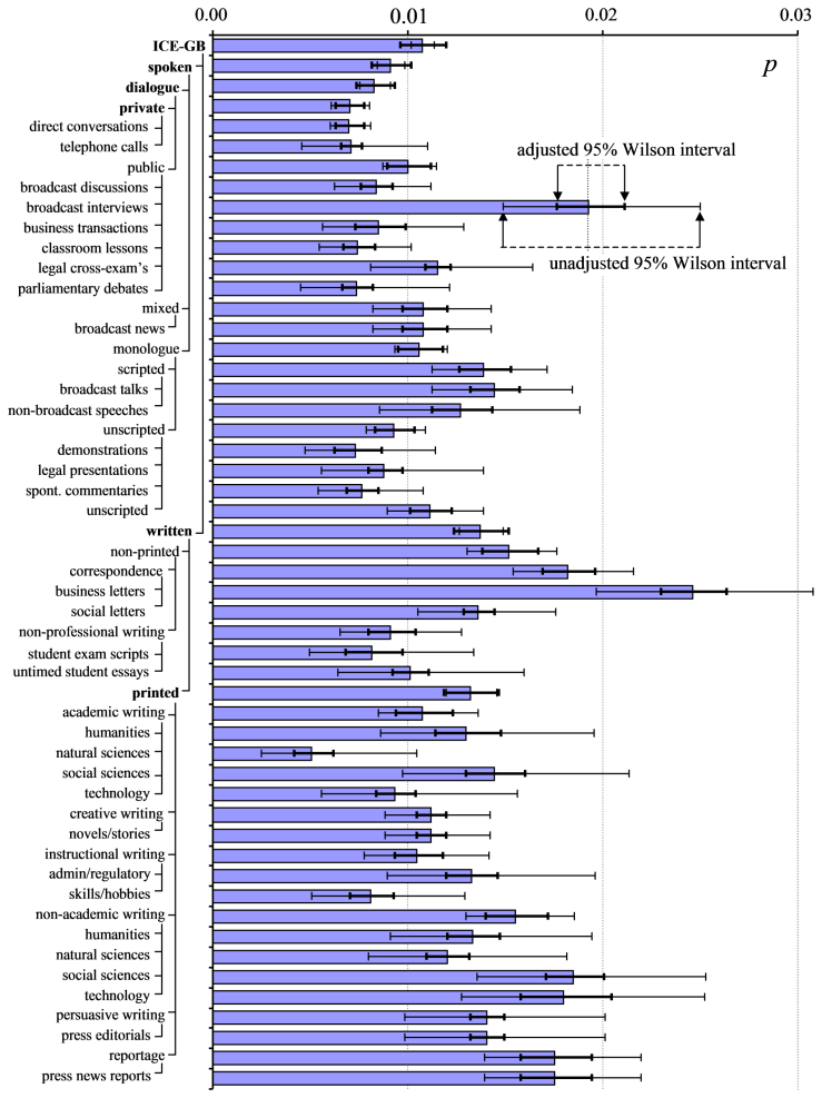
The figure reinforces observations we made earlier. Within a single text type, such as broadcast interviews, p has a compressed range and cannot plausibly approach 1. (Note that mean p does not exceed 0.03 in any genre.) The observed between-text distribution is smaller than that predicted by Equation (3), and, armed with this information, we are able to reduce the 95% Wilson score interval for p. This degree of compression (or, to put it another way, the plausible value of max(p)) may also differ by text genre.
However, the reduction due to range-compression is offset by a countervailing tendency: pooling genres increases the variance of p. The distribution of texts across the entire corpus consists of the sum of the spoken and written distributions (means 0.0091 and 0.0137 respectively), and so on.
The Wilson interval for the mean p averaged over all of ICE-GB approximately doubles in width (Fss = 0.2509), and the intervals for spoken, dialogue, written and printed (marked in bold in Figure 6) also expand, albeit to lesser extents. The other intervals contract (Fss > 1), tending to generate a more consistent set of intervals over all text categories.
Contents
- Introduction
- Previous research
2.1 Employing rank tests2.2 Case interaction models
- Adjusting the Binomial model
- Example 1: interrogative clause probability, direct conversations
4.1 Alternative method: fitting
- Example 2: Clauses per word, direct conversations
- Uneven-size subsamples
- Example 3: Interrogative clause probability, all ICE-GB data
- Example 4: Rate of transitive complement addition
- Conclusions
Citation
Wallis, S.A. 2015. Adapting random-instance sampling variance estimates and Binomial models for random-text sampling. London: Survey of English Usage, UCL. www.ucl.ac.uk/english-usage/statspapers/recalibrating-intervals.pdf
Citation (extended version)
Wallis, S.A. 2021. Adjusting Intervals for Random-Text Samples. Chapter 17 in Wallis, S.A. Statistics in Corpus Linguistics Research. New York: Routledge. 277-294.
References
Sheskin, D.J. 1997. Handbook of Parametric and Nonparametric Statistical Procedures. Boca Raton, Fl: CRC Press.
Wallis, S.A. 2013. Binomial confidence intervals and contingency tests: mathematical fundamentals and the evaluation of alternative methods. Journal of Quantitative Linguistics 20:3, 178-208 » Post
