This post is a little off-topic, as the exercise I am about to illustrate is not one that most corpus linguists will have to engage in.
However, I think it is a good example of why a mathematical approach to statistics (instead of the usual rote-learning of tests) is extremely valuable.
Case study: The declared ‘deficit’ in the USS pension scheme
At the time of writing (March 2018) nearly two hundred thousand university staff in the UK are active members of a pension scheme called USS. This scheme draws in income from these members and pays out to pensioners. Every three years the pension is valued, which is not a simple process. The valuation consists of two aspects, both uncertain:
- to value the liabilities of the pension fund, which means the obligations to current pensioners and future pensioners (current active members), and
- to estimate the future asset value of the pension fund when the scheme is obliged to pay out to pensioners.
What happened in 2017 (and happened in the last two valuations) is that the pension fund has been declared to be in deficit, meaning that the liabilities are greater than the assets. However, in all cases this ‘deficit’ is a projection forwards in time. We do not know how long people will actually live, so we don’t know how much it will cost to pay them a pension. And we don’t know what the future values of assets held by the pension fund will be.
The September valuation
In September 2017, the USS pension fund published a table which included two figures using the method of accounting they employed at the time to value the scheme.
- They said the best estimate of the outcome was a surplus of £8.3 billion.
- But they said that the deficit allowing for uncertainty (‘prudence’) was –£5.1 billion.
Now, if a pension fund is in deficit, it matters a great deal! Someone has to pay to address the deficit. Either the rules of the pension fund must change (so cutting the liabilities) or the assets must be increased (so the employers and/or employees, who pay into the pension fund must pay more). The dispute about the deficit engulfed UK universities in March 2018 with strikes by many tens of thousands of staff, lectures cancelled, etc. But is there really a ‘deficit’, and if so, what does this tell us?
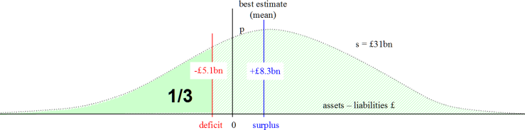
The first additional bit of information we need to know is how the ‘uncertainty’ is modelled. In February 2018 I got a useful bit of information. The ‘deficit’ is the lower bound on a 33% confidence interval (α = 2/3). This is an interval that divides the distribution into thirds by area. One third is below the lower bound, one third above the upper bound, and one third is in the middle. This gives us a picture that looks something like this:
Of course, experimentalist statisticians will never use such an error-prone confidence interval. We wouldn’t touch anything below 95% (α = 0.05)! To make things a bit more confusing, the actuaries talk about this having a ‘67% level of prudence’ meaning that two-thirds of the distribution is above the lower bound. All of this is fine, but it means we must proceed with care to decode the language and avoid making mistakes.
In any case, the distribution of this interval is approximately Normal. The detailed graphs I have seen of USS’s projections are a bit more shaky (which makes them appear a bit more ‘sciency’), but let’s face it, these are projections with a great deal of uncertainty. It is reasonable to employ a Normal approximation and use a ‘Wald’ interval in this case because the interval is pretty much unbounded – the outcome variable could eventually fall over a large range. (Note that we recommend Wilson intervals on probability ranges precisely because probability p is bounded by 0 and 1.)
What do we know?
- The best estimate is the median of the distribution. In the case of the Normal it is also the mean, v = 8.3 (billion pounds).
- The lower bound of the confidence interval v– = –5.1. This is the quoted deficit figure.
- The error level of the Normal distribution α = 2/3.
- The critical value of the Normal distribution, zα/2 = 0.4307.
We also know that v– = v – zα/2.s.
- So we can calculate the standard deviation s = (v – v–) / zα/2 = 31.1101.
That’s a standard deviation of £31 billion! No wonder the Normal distribution looks so wide.
This tells us that a big problem with the prediction is the sheer scale of the uncertainty attached to the estimate. It is not necessarily a problem with the pension – after all, even using this valuation method it is odds-on to reach a positive outcome of £8.3 billion.
Now, it turns out that there are lots of problems with the method for valuing the pension scheme. Crucially, the entire exercise is predicated on imagining the ‘old’ UK universities (or a large proportion of them) go bankrupt. I have written about this elsewhere. It is not crucial for our statistics discussion, even if it is a costly problem for staff, employers and students impacted by the industrial action as the argument about who should pay for this type of ‘deficit’ ensues.
Irrespective of the rights and wrongs of that argument (and we will return to this in conclusion), this exercise should have convinced you of one thing though – with such a high level of uncertainty about the valuation, pretty much any value can be obtained!
The probability of default
The next thing I did was wonder, what is the break-even (zero) point on the distribution, where valuation v = 0? In other words, can we calculate the chance of default occurring according to this model?
This seems to me to be an important operation. Most of all it allows us to meaningfully compare different valuations, which, as we shall see in a minute, is a useful thing to do. The USS Trustees, who manage the scheme, are concerned with one thing – the risk of default, p(v < 0). So it strikes me that we ought to calculate it.
The zero point is the value of α/2 when v– = v – zα/2.s = 0.
So we need to know α when zα/2 = v/s = 0.2667.
There are various ways to compute this, but I used a poor-man’s Newton-Raphson method in Excel to find α. That is, I input different values of α until the Normal function (‘NORMSINV(1-(α/2))’) obtained a closely-similar value of z!
I am sure there is a neater way, but it would obtain essentially the same result. It’s the maths that count!
- In this case, this obtains error level α = 0.79.
This means that there would be an area of 0.21 inside the interval if v– = 0. Another way of thinking about this is that, of the half-distribution below the mean, 21% of that area is where v ≥ 0.
So we can now report that the probability of default p(v < 0) = 0.5 – 0.21/2 = 0.395.
The November valuation
As a result of the valuation in September there was much shaking of heads amongst employers. This level of risk seemed to great to bear. So they reported to their organisation, Universities UK (UUK) that they wanted to see less risk in their model. The first valuation employed a method that was termed gradual ‘de-risking’, meaning that the assets would be moved from a mixed stocks and shares portfolio into investments in government stocks, termed ‘gilts’. The idea is that this is less risky because these gilts are ‘low risk’ compared to stocks and shares.
As a result of this consultation, the scheme actuaries were sent away and they came up with some different figures. These were
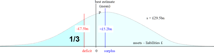
- The best estimate, v = £5.2bn (this figure was not made very public)
- The quoted deficit, v– = -£7.5bn (this was made very public)
Again, the same interval calculation was employed.
I was ‘leaked’ the best estimate. Knowing now how the calculation was made for our first valuation, I employed the same method.
- The standard deviation s = (v – v–) / zα/2 = 29.4850.
The graph now looks like this.
So, what is the probability of default, i.e. p(v < 0)? What has happened to the risk to the Pension Trustees?
We have zα/2 = v/s = 0.1764, which obtains α = 0.86.
- The probability of default, p(v < 0), is now 0.43.
‘De-risking’ increases the risk of default
So – wait for this – if the employers engage in what they think is a ‘risk-averse’ modelling approach, they increase the risk of default! What is going on?
Let’s pause for a moment.
- The risk of default is an estimated risk of the likely outcome of the unravelling of the pension scheme should this prove necessary. It is like predicting the chance of an aeroplane crashing.
- But the ‘risk’ of stock-market investments is a different thing entirely. It is volatility, short-term variation, that might increase or decrease investments over the short term. To use our aeroplane analogy, it is turbulence.
- What the November valuation did was drop the altitude of the plane to avoid turbulence, but it increased the risk of crashing the plane into mountains!
People are not used to reasoning with probability and risk, and it is easy to conflate different probabilities and different risks. Only a logical and mathematical approach to thinking about probability can rescue you from the kind of error exhibited by the university employers, when, insisting on a ‘lower level of risk’, they managed to increase the risk to the scheme and themselves.
What is quite disturbing about this argument is that I am not a professional actuary, yet I spotted the error immediately. I was not the only one.
You would think that the first thing a competent professional would do on obtaining this new calculation is critique it, wonder why this counter-intuitive outcome had been obtained, and advise those running the scheme accordingly. Yet at the time of writing in March 2018, UUK are still trying to use this November valuation to try to get their way.
So-called ‘de-risking’ increases the only risk that should matter (the risk of ultimate default), and therefore it is neither a competent investment strategy nor a good method for valuing the pension scheme!
What happens if no de-risking is applied at all?
Here we don’t have published figures from USS. But we have some information from our previous calculations.
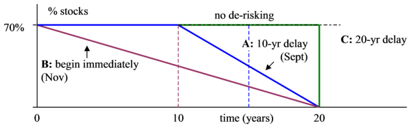
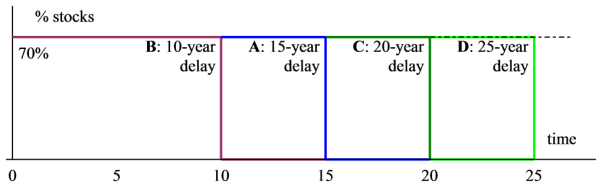
The September valuation was obtained, not by employing no de-risking, but by modelling the effect of replacing stocks and shares with gilts after a 10 year-delay. The November valuation was obtained by starting de-risking immediately. Both aim for complete de-risking by the 20-year point. See Figure 3.
We also can safely assume that the cost and yield of gilts is likely to be stable. (Indeed the low ‘long term gilt yield’ is half the problem of valuing live pension schemes like this.)
In the first place we have two valuations, A (September) and B (November).
These can be depicted like this.
We can now estimate the likely outcome for a new model, C, that employs a 20-year delay before total divestment, using some simple maths and the Bienaymé theorem (that independent variances may be summed).
Gilts are predicted to have a more-or-less constant low value. Stocks are predicted to be more volatile, around a given mean growth rate.
If we assume that stocks continue to perform in a similar manner over each five-year period (i.e. that the best estimate and standard deviation of the growth rate is constant) the areas under the curve for A and B are equivalent to immediate and total divestment at time points 15 and 10 years respectively (dashed vertical lines). This is because we can assume that the exposure of assets to stock market risk is considered to be constant.
Consider B first. This employs an immediate de-risking model which has the lowest standard deviation and variance.
- Var(B) = s1² = 869.36
In the case of A, there is an additional variance term due to the stocks-and-shares uncertainty generated by delay:
- Var(A) = s1² + s2² = 967.84
Therefore the additional uncertainty due to delayed de-risking s2² = 967.84 – 869.36 = 98.48.
Assuming investment performance, gilt yields, etc. are constant over time, the area between A and B is also the same area between A and C.
- Var(C) = s1² + 2s2² = 1,066.32,
- Standard deviation for C, s = 32.6545.
We obtain the best estimate for C by simple addition, so v = £11.4 billion.
This gives us a ‘deficit’ of –£2.66 billion and a probability of default of 0.3635.
Moving to an ongoing valuation
Note that the gradual de-risking model (A) is roughly equivalent to delaying de-risking for five years and then selling stock as in model B. We can now compute D (25-year delay), E (30-year delay), and further models employing the same approach.
This obtains the following graphs.
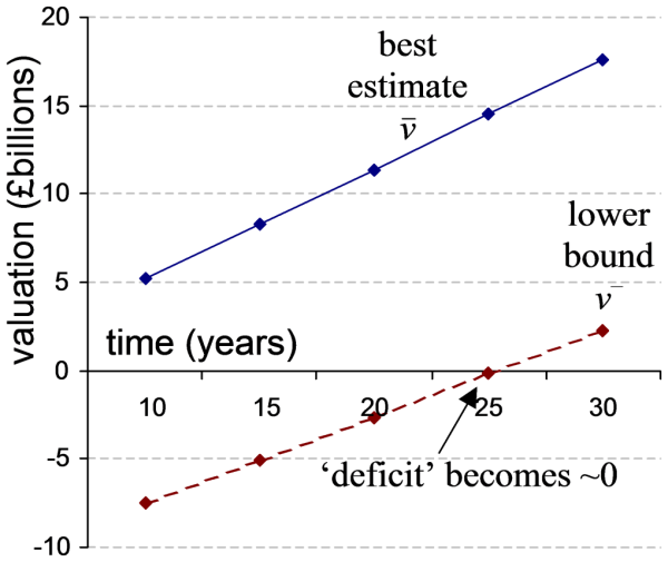
In other words, even if one agreed to de-risk in twenty-five years’ time, the projected deficit would be close to zero, and thereafter, the scheme generates a surplus at this level of prudence.
Therefore not de-risking at all (performing an ongoing valuation) must obtain a surplus. The limit of this ‘deficit’ curve exceeds zero.
If long-term gilt yields rise beat CPI, then the benefits of increased predictability might outweigh the loss in asset performance. But we would need to perform a calculation of the trade-off based on the best evidence available at the time. What is clear is that de-risking punishes the pension scheme for an external factor – low long-term gilt and bond yields – for no good reason.
Another way to see the same result is to plot the probability of default over these different ‘de-risking horizons’. This obtains the following graph of p(v < 0).
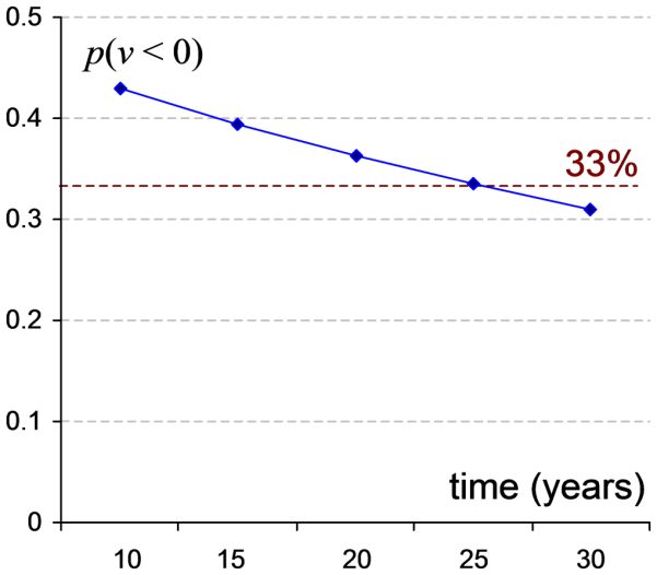
The evidence is therefore that an assessment of the assets and liabilities of the live pension scheme (an ‘ongoing valuation’) must return a net surplus. Indeed, this is what the actuaries First Actuarial found by other methods (Salt and Benstead 2017).
Some might object that there were other differences between the November and September valuations, and therefore taking the difference between them is not appropriate. This may be true, but the burden of evidence has shifted. Until actuaries working for UUK and USS are transparent about their assumptions, I would suggest that I have demolished the idea that there could be an ongoing deficit by a straightforward mathematical argument.
In conclusion
The ability to conceptualise probability in a meaningful way is central to any rational argument about statistics and uncertainty. We can see this in the confusion between ‘de-risking’ and real risk, i.e. risk of pension default.
There is one last sting in this particular tale.
In the case of the USS pension, the entire premise of ‘de-risking’ is that a trigger event as financially destabilising to the bankruptcy of the entire pre-92 university sector takes place. This might not mean the total bankruptcy of the sector, but it would require a large number of big institutions to shut down and the remaining institutions to fail to absorb their students, staff and market share.
Now, the probability of this event is – or should be – effectively zero. Since p(v < 0) × 0 = 0, from a logical perspective it does not really matter what the probability of deficit actually is. However, the current UK regulatory environment still presumes that pension funds must be evaluated by ‘managing the risk of default’ (which means in practice modelling by de-risking), even if the probability of the trigger event is zero.
That an evaluation of this kind is even contemplated in the case of USS illustrates what one might call a wilful ignorance of basic mathematics. One of the Big Four accountancy firms has attached their name to various tendentious statements about the USS pension scheme, levels of prudence, etc. It is to their shame that they have done so.
As we have demonstrated, the probability of scheme default is zero provided that the scheme is not de-risked. Actual de-risking – an act of self-harm of the first order – increases the chance of default, although even in the worst case, immediate de-risking is still odds-on to leave a surplus.
The obvious solution to the current crisis is for the Government to accept that a multi-employer scheme of publicly-funded universities is not subject to the same risks of a single-employer pension fund.
Sector bankruptcy would be a national tragedy that would also constitute the simultaneous collapse of one of the UK’s leading exporting industries (higher education), the eviction of millions of students from their courses and the collapse of the UK independent research sector. It is a political issue of the utmost importance to the UK economy as well as generations of university staff and students.
Cuts in the pension benefits and increases in employer expenditure are pointless and damaging when the ‘deficit’ is so obviously an artefact of the valuation method. The obvious solution is that the Government simply guarantees the security of the pension fund, and permits the Trustees to value the scheme on an ongoing basis.
Footnote 1 (October 2018)
Sam Marsh uncovers that the trigger reasoning used by the pension fund USS for deciding to ‘de-risk’ (‘Test 1’) contains a colossal error. Even if the Government did not step in, USS itself has no grounds to ‘de-risk’. See also Mike Otsuka’s explanation.
Footnote 2 (December 2019)
In 2019, USS Ltd and the employers’ organisation, UUK, changed approach. Instead of threatening to reduce future benefits to employees, they proposed increasing contributions from employers and employees. Based on 2018 contribution rates of £2.2bn pa, we would expect these additional contributions (3.1% from employers and 1.6% from employees) to yield £0.83bn over the 2 years to the next valuation round.
However, in fact, the USS asset portfolio grew in value by £7.4bn between 2017 to 2019. Although the scheme is being valued as if it were ‘de-risked’, in the real world the assets remained in stock investments and increased in value substantially. (Clearly, this £7.4bn figure of actual growth dwarfs any small increase that might be obtained by increased contributions.) Only ~£0.4bn of this figure was added by excess contributions.
CPI inflation from September 2017 to 2019 was 4.4% compounded.
Even if the scheme were de-risked, using Model A valuation assumptions above, the liabilities in 2017 were £65.1bn. These can be uprated by CPI, giving us £65.1bn × 1.044 = £68bn. This leaves us with a deficit of £0.6bn at most, which can be addressed by other minor scheme changes, smoothing etc. as the Joint Expert Panel proposed.
The only justification now used for making changes is to employ immediate and irrevocable de-risking (Model B). Figures released by USS in the valuation update show a growing deficit whose only explicable cause is continued application of the absurd Model B. Employing this strategy creates a perpetual crisis.
There is no need for any changes to the scheme, whether by increasing contributions or reducing benefits. On the other hand de-risking voluntarily undermine the very stability of the pension scheme.

Reblogged this on Let's Look at the Figures and commented:
Following a recent Twitter exchange with Ian Dryden, I was thinking I’d write something about the risk of default for the USS pension scheme. But then I came across this other new post at corp.ling.stats — which has already done what I was intending!
I believe this to be a very cogent contribution to the debate. Moving pension assets into gilts may reduce money value certainty but increases real value uncertainty and decreses expected return. USS projections should publish all assumptions and methods. It is also not clear that funds should be actively managed although (suprise, suprise) the active managers think they should be.
Reblogged this on Dov Stekel's Laboratory and commented:
This is great and well worth reading!