The other end of the telescope

Introduction

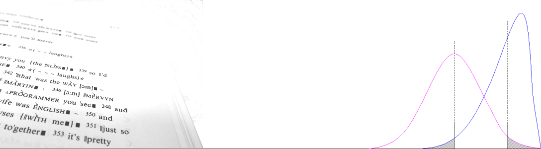
The standard approach to teaching (and thus thinking about) statistics is based on projecting distributions of expected values. The distribution of an expected value is a set of probabilities that predict the relative chance of each possible value, according to a mathematical model of what you predict should happen.

For example, the Binomial model predicts the chance of obtaining f instances of a type, A, drawn from n instances of two types, A and B, assuming each instance in the sample is independent from the next, the population is infinite in size, and any random instance could be either A or B.

For the experimentalist, this distribution is the imaginary distribution of very many repetitions of the same experiment that you have undertaken. It is the output of a mathematical model.

• Note that this idea of a projected distribution is not the same as the ‘expected distribution’. An expected distribution is a series of values you expect your data should match, according to your null hypothesis.
• Thus in what follows we simply compare a single expected value P with an observed value p. This can be thought of as comparing the expected distribution E = {P, 1 – P} with the observed distribution O = {p, 1 – p}.

Thinking about this projected distribution represents a colossal feat of imagination: it is a projection of what you think would happen if only you had world enough and time to repeat your experiment, again and again. But often you can’t get more data. Perhaps the effort to collect your data was huge, or the data is from a finite set of available data (historical documents, patients with a rare condition, etc.). Actual replication may be impossible for material reasons.

In general, distributions of this kind are extremely hard to imagine, because they are not part of our directly-observed experience. See Why is statistics difficult? for more on this. So we already have an uphill task in getting to grips with this kind of reasoning.

Significant difference (often shortened to ‘significance’) refers to the difference between your observations (the ‘observed distribution’) and what you expect to see (the expected distribution). But to evaluate whether a numerical difference is significant, we have to take into account both the shape and spread of this projected distribution of expected values.

When you select a statistical test you do two things:

• you choose a mathematical model which projects a distribution of possible values, and
• you choose a way of calculating significant difference.

The problem is that in many cases it is very difficult to imagine this projected distribution, or — which amounts to the same thing — the implications of the statistical model.

When tests are selected, the main criterion you have to consider concerns the type of data being analysed (an ‘ordinal scale’, a ‘categorical scale’, a ‘ratio scale’, and so on). But the scale of measurement is only one of several parameters that allows us to predict how random selection might affect the sampling of data.

A mathematical model contains what are usually called assumptions, although it might be more accurate to call them ‘preconditions’ or parameters. If these assumptions about your data are incorrect, the test will probably give an inaccurate result. This principle is not either/or, but can be thought of as a scale of ‘degradation’. The less the data conforms to these assumptions, the more likely your test is to give the wrong answer.

This is particularly problematic in some computational applications. The programmer could not imagine the projected distribution, so they tweaked various parameters until the program ‘worked’. In a ‘black-box’ algorithm this might not matter. If it appears to work, who cares if the algorithm is not very principled? Performance might be less than optimal, but it may still produce valuable and interesting results.

But in science there really should be no such excuse.

The question I have been asking myself for the last ten years or so is simply can we do better? Is there a better way to teach (and think about) statistics than from the perspective of distributions projected by counter-intuitive mathematical models (taken on trust) and significance tests?

Why is statistics difficult?

Imagine you are somewhere on a road that you have never been on before. Picture it. It’s peaceful and calm. A car comes down the road. As it gets to a corner, the driver appears to lose control, and the car crashes into a wall. Fortunately the driver is OK, but they can’t recall what happened.

Let’s think about what you experienced. The car crash might involve a number of variables an investigator would be interested in.

• How fast was the car going? Where were the brakes applied?
• Look on the road. Get out a tape measure. How long was the skid before the car finally stopped?
• How big and heavy was the car? How loud was the bang when the car crashed?

These are all physical variables. We are used to thinking about the world in terms of these kinds of variables: velocity, position, length, volume and mass. They are tangible: we can see and touch them, and we have physical equipment that helps us measure them.